Abstract
A proof assistant checks a computation by reducing it, so the data structure a
verified algorithm is written over decides the cost of being checked, not only
the cost of running. This paper measures that cost for one task with a locked
specification: counting the partitions of n in Lean 4, where the answer must
come with a machine-checked proof that holds for every n. Three designs
compute the same recurrence. Evaluating the specification as written performs
672,182 primitive steps at n = 36, because every path to a table cell
re-derives it. Holding each table row as a list brings that to 69,768, since
a cell is then looked up rather than recomputed, but indexing position m of a
list costs m constructor matches. Holding the whole row in a single natural
number, with the entry for m in the m-th field of w bits, brings it to
716: a factor of 939 against the specification and 97 against the lists,
and in reduction wall time 57.64 seconds against 0.07. The representation is
sound only if no field overflows, which is a theorem and not an assumption:
peeling one term off the specification’s own sum yields
partAux (k+1) m = partAux k m +
partAux (k+1) (m - (k+1)), from which
partAux k m ≤ 2m+k follows, so w = 2n+1 bits suffice. The
development uses core Lean only and proves its statement for every n. Asking
the same question of the other seven problems found something the packing does
not address: two of the eight shipped reference starters cannot be reduced at
any judged size, both reaching well-founded recursion through
Nat.minFac, so both score nothing while compiling with correct
proofs. The competition’s own metric has since scored
this entry at 131,460,833 units against 3,396,012,941 for a
narrow-operand alternative proved the same way, a factor of 25.8. The step
count is blind to a field-width tuning worth a further 3.4 in wall time. Code and data are public.
Introduction
A program that is merely run can be as clever as its author likes. A program that must be checked is different, because something else now has to follow it, and that something else is usually much simpler than the program.
In Lean 4, the checker is the kernel [2]. To accept a proof that some
closed term equals some value, the kernel reduces the term. It does this with a
small and deliberately unadventurous evaluator: it unfolds definitions, matches
constructors, and calls out to arbitrary-precision integer arithmetic for the
primitive operations on Nat. There is no compiler, no register
allocator and no memoisation. Work the kernel repeats is work nobody can
optimise away, because the kernel is the thing whose simplicity is the point
[5].
That gives an unusual shape to the question of which data structure to use. In ordinary programming, the choice between an array and a list is a choice about how fast the program runs. Here it is a choice about how much work the kernel must perform to be convinced, and the two are not the same quantity. A representation can be excellent to compute with and terrible to check, because the operations the kernel charges for are not the operations a processor charges for.
This paper takes one task where that tension is sharp and measures it. The task
is the partition problem of the SAIR Lean Kernel Challenge
[1]: given n, produce the number of partitions of n, together with a
Lean proof that the produced function agrees with a specification the
competition fixes in advance. The specification is a recurrence with
overlapping subproblems, which makes it the smallest interesting case of a
general situation: a dynamic program that has to be checked rather than merely
run.
**The idea.**Figure 1 is the whole of the contribution in one picture. A table
row held as a list is a chain, and reaching the m-th entry means walking m
links, which the kernel charges for one link at a time. The same row held as
the digits of a single natural number in base 2w is one object, and reaching
the m-th entry is a shift and a mask: two operations, whatever m is.
Arithmetic on that one object then does to the whole row at once what the
recurrence says to do to each entry.
Figure 1. The two representations of one table row. Both hold the same numbers. The list charges the kernel for the distance to an entry; the packed row does not, because the entry's position is an exponent rather than a path. Everything else in this paper follows from that difference, including the one theorem the packed row needs and the list does not.
**Why the theorem is not optional.**Packing is not free of obligations. Fields sit next to each other in one integer, so if any entry ever needs more than w bits it carries into its neighbour, and the neighbour is then silently wrong. No type error reports this and no test at small n need reveal it. The representation is therefore correct only relative to a bound on the values it holds, and Section 4 proves that bound from the specification itself rather than assuming it. It is the only thing standing between this design and a wrong answer that is fast. Contributions.
- A representation for kernel-checked dynamic programming that carries a
whole table row in one
Nat, and a row step that is the specification’s own sum lifted to that representation rather than a new recurrence to be justified separately (Section 3). - The bound partAux k m ≤ 2m+k, proved in Lean from a peeling identity on the specification’s sum, which is what licenses the packing and fixes the field width at 2n+1 bits (Section 4).
- A correctness proof that is universal in n rather than checked on the
judged range, self-contained in core Lean, and resting only on
propextandQuot.sound(Section 5). - A measurement of all three designs under two metrics, an operation count derived from the definitions and wall time measured in continuous integration, together with a statement of where the two disagree and why (Section 6).
The task
The specification, and why it is locked
The competition fixes the specification and forbids changing it [1]. In Lean:
partAux 0 0 = 1
partAux 0 (n+1) = 0
partAux (k+1) m = Σj=0⌊ m/(k+1)⌋
partAux k (m - j (k+1))
partitionSpec n = partAux n n
An entry supplies a function impl and a proof of
∀ n, impl n = partitionSpec n.
(1)
The quantifier is the competition's, and it matters. A proof for the six sizes that are scored would be a much weaker statement and a much easier one; the requirement is a single theorem covering every natural number, including 0 and sizes no machine will ever evaluate.Two further rules shape what an entry may do. The proof must rest only on
propext, Quot.sound and Classical.choice, which
excludes sorry and, more pointedly, excludes
native_decide: that tactic discharges a goal by compiling and
running it outside the kernel, adding an axiom that asserts the compiler agreed
[3]. It is fast and it is exactly the shortcut this task exists to
forbid, because it moves the computation out of the thing whose trust is being
measured. And partial and unsafe definitions are excluded,
so every function must be seen to terminate.
What is being ranked
Rank is the total hardware instruction count the kernel spends reducing
impl n over six hidden cases, with n between 14 and 36
[1]. Instruction count rather than time is the right choice for a
competition, since it is nearly free of scheduling noise, but it is read through
perf_event_open against the hardware performance counters, and a
virtualised continuous-integration runner does not expose those. Every number
this paper reports is therefore either an operation count derived from the
definitions or a wall time, and Section 6 keeps the two apart.
Why the specification is expensive to evaluate
Equation (2.1) has overlapping subproblems, and nothing in the definition shares them. Reducing partitionSpec 36 by unfolding performs 128,553 calls to partAux, for a table that contains only 37 × 37 = 1,369 distinct cells. The waste is not incidental; it is the entire difficulty of the problem, and every design below is a different answer to the question of where to put the values so they are computed once.
Three designs
All three designs compute the recurrence of Section 2 without altering it, and differ only in where the intermediate values are kept.
The specification as written
Taking impl = partitionSpec satisfies
equation (1) by rfl, which is the cheapest possible proof
and the most expensive possible computation. It is included here as the
baseline, because it is what the difficulty is measured against.
Memoisation by rows of lists
The first real design keeps a row of the table as a List Nat, builds
row k+1 from row k, and names the previous row once so that it is built
once:
def rows : Nat -> Nat -> List Nat
  | 0,     len => baseRow len
  | k + 1, len => let prev := rows k len
                  nextRow (k + 1) prev len
The design’s useful property is in how nextRow is written. Rather than stating a new recurrence over lists and proving it equivalent to the specification, it reuses the specification’s own inner sum with the recursive call abstracted out:
def specSum (g : Nat -> Nat) (d m : Nat) : Nat :=
  ((List.range (m / d + 1)).map (fun j => g (m - j * d))).foldl (+) 0
so that partAux (k+1) m and specSum (partAux k) (k+1) m are literally the same term. Correctness of the whole table then reduces to a congruence: two functions that agree everywhere the sum looks give the same sum, and the sum only ever reads indices m - jd ≤ m. That is a three-line induction rather than a re-derivation of the recurrence, and the same discipline carries over unchanged to the packed design in Section 3.3.
What this design pays for is indexing. Reading position m of a list walks m cons cells, and the sum at cell m of row d reads positions m - jd for every j, so the cost of the whole table is
Σd=1n Σm=0n Σj=0⌊ m/d ⌋ (m - jd + 1)
(2)
constructor matches, which is 51,353 at n = 36 before any arithmetic is counted. The values are computed once, and then walked to many times. ### One row in one natural number The second design changes only where the values live. Fix a field width w and hold row k as the single natural number whose m-th base-2w digit is partAux k m:pack w f ℓ = Σm=0ℓ - 1 f(m) 2wm,
(3)
defined in Lean by the recursion pack w f (ℓ+1) = f 0 + 2w· pack w (f ∘ (· + 1)) ℓ, with pack w f 0 = 0. Reading field m is then ⌊ R / 2wm ⌋ mod 2w: one shift and one mask, independent of m. That is the whole of what the change buys, and Figure 1 is a picture of it. Carrying several table entries in the fields of one integer is an existing idiom, credited in Section 8; what does not come with it is the obligation of Section 4, which arbitrary precision creates and a machine word removes.The interesting part is that the row step needs no new idea either. Write R for row k and let d = k+1 be the largest part the next row admits. Then
R' = ( R + (R ≪ dw) + (R ≪ 2dw) + … + (R ≪ ⌊ n/d⌋ dw) ) mod 2w(n+1)
(4)
is row k+1, because field m of the sum in equation (4) isΣj : jd ≤ m (field m - jd of R) = Σj=0⌊ m/d ⌋ partAux k (m - jd),
(5)
which is exactly the right-hand side of equation (2.1). Shifting by jdw moves field m - jd into position m; adding the shifted copies performs the specification's sum over multiplicities in every field at once; and the outer modulus discards the fields above n, which the shifts have filled with values belonging to a longer row. Figure 2 shows one step.Figure 2. One row step of equation (4) with d = 2, drawn for a row of seven fields. Each shifted copy contributes the entry d places to the left, which is the term for one more copy of the part d. The kernel performs each shifted copy as one operation on one large integer, so the number of operations depends on ⌊ n/d ⌋ and not on how many fields the row has. Each field of R' carries one term per copy that reaches it, so fields 0 and 1 carry one, fields 2 and 3 carry two, and fields 4 to 6 carry three.
The operation count follows directly. The sum in equation (4) has ⌊ n/d ⌋ shifted terms, so over all rows the design performsΣd=1n ⌊ (n)⁄(d) ⌋ = 140 (n = 36)
(6)
shift-and-add pairs, against the 51,353 constructor matches of equation (2). Equation (6) is a harmonic sum, so the packed count grows as n ln n. Fitting a power law to the measured counts over 14 ≤ n ≤ 36 gives an exponent of 1.14 for the packed row against 2.68 for the lists and 5.33 for the specification as written, so the gap widens with n rather than holding, which Section 6 confirms in wall time as well. ## The bound that licenses the packing Equation (4) is only row k+1 if the additions in it stay inside their fields. If some entry reaches 2w it carries into the field above, corrupting a neighbour, and the corruption propagates through every later row. The design is therefore correct only relative to a bound on the table's values, and the bound has to be proved rather than observed, because observing it at the judged sizes says nothing about equation (1), which is universal. ### A peeling identity The usable form of the specification is not equation (2.1) but a one-step version of it. > **Lemma 1 (Peeling).** For m ≥ k+1, > >partAux (k+1) m = partAux k m + > partAux (k+1) (m - (k+1)).
>(7)
Proof. Write d = k+1. By equation (2.1), partAux d m = Σj=0⌊ m/d⌋ partAux k (m - jd). Separating the j = 0 term leaves Σj=1⌊ m/d⌋ partAux k (m - jd), and substituting j = i + 1 turns that into Σi=0⌊ m/d⌋ - 1 partAux k ((m - d) - id). Since m ≥ d we have ⌊ m/d ⌋ - 1 = ⌊ (m-d)/d ⌋, so the remaining sum is exactly partAux d (m - d) by equation (2.1) again. □ Combinatorially equation (7) says that a partition of m into parts at most d either uses no copy of d, or uses at least one and leaves a partition of m - d. The reason to prefer it to equation (2.1) is that it replaces a sum of unknown length with two terms, which is what makes an induction possible.
The bound
Proposition 2. For all k and m, partAux k m ≤ 2m+k.
Proof. By induction on k, and for each k by induction on m.
For k = 0: partAux 0 0 = 1 = 20 by equation (2.1), and partAux 0 (m+1) = 0 by equation (2.1).
For k+1, suppose the claim holds for k at every argument, and for k+1 at every argument below m. If m < k+1 then ⌊ m/(k+1) ⌋ = 0, so equation (2.1) gives partAux (k+1) m = partAux k m ≤ 2m+k ≤ 2m+k+1. If m ≥ k+1 then Lemma 1 applies, and
partAux (k+1) m ≤ 2m+k + 2(m - (k+1)) + (k+1) = 2m+k + 2m ≤ 2m+k + 2m+k = 2m+k+1,
(8)
where the first summand uses the outer hypothesis at k and the second the inner hypothesis at m - (k+1) < m. □
Corollary 3. If k ≤ n and m ≤ n then partAux k m ≤ 22n < 22n+1, so a field width of w = 2n+1 bits holds every entry of every row without carry. Two things about Proposition 2 are worth being explicit about. The first is that it is loose, and known to be: at n = 36 the bound reserves 73 bits for values that never exceed 17,977, which needs 15. The slack is visible in equation (8), where the second summand is raised from 2m to 2m+k so that the two terms combine into a single power. The second is that looseness here costs almost nothing, for a reason Section 6.4 takes up: a wider field makes each operand larger but does not change how many operations there are. The bound was chosen to be easy to prove rather than tight, and that was the right trade, but it was a trade and not a free choice. An earlier version used w = n⌈ log2 (n+1)⌉ + 1, which is 217 bits at n = 36, and replacing it with 2n+1 was measured at a factor of 3.4 in wall time.
How loose, measured
Calling a bound loose is a claim with a number attached, so Table 1 attaches it. For each judged size the table gives the largest value the table actually holds, the bits that value needs, and the bits each candidate width reserves. The proved bound reserves between 3.6 and 4.9 times the bits required, and the ratio grows with n.
The table also discharges two things a reader would otherwise take on trust. Proposition 2 is checked at every one of the (n+1)2 cells at every judged size rather than spot-checked, and so is the tighter bound of Proposition 4 below, which the paper recommends but does not prove in Lean. Recommending an unproved bound that turned out to fail somewhere would be worse than not recommending one.
Proposition 4. For all k and m, partAux k m ≤ 2m (k+1).
Proof. By the same nested induction as Proposition 2. For k = 0 the value is 1 or 0 and 2m ≥ 1. For k+1 with m < k+1, equation (2.1) gives partAux (k+1) m = partAux k m ≤ 2m(k+1) ≤ 2m(k+2). For m ≥ k+1, Lemma 1 and the two hypotheses give
partAux (k+1) m ≤ 2m(k+1) + 2m-(k+1)(k+2) ≤ 2m(k+1) + 2m = 2m(k+2),
(9)
using 2m-(k+1)(k+2) ≤ 2m, which holds because k+2 ≤ 2k+1. □ Proposition 4 gives a field of m + ⌈log2(k+1)⌉ bits, which is 42 at n = 36 against the 73 of Corollary 3: a factor of 1.7 narrower, and still 2.8 times wider than the 15 bits any cell needs. It is not in the submitted file because the arithmetic step in equation (9) needs the auxiliary fact k+2 ≤ 2k+1, which is a second induction, and the entry was already closing. | | || | | | | | | | | | | | | | |
Table 1. What the bound reserves against what the table needs. The fourth column is the width used before Proposition 2 was proved, the fifth is Corollary 3, and the sixth is Proposition 4. The waste column is the fifth divided by the third, the price actually paid for a bound chosen to be easy to prove. Both bounds were verified at every cell at every size by tools/bound_slack.py, which fails rather than reports if either is violated anywhere.
Correctness in Lean
The entry proves equation (1) in the form ∀ n, impl n = partitionSpec n, by the same congruence argument the list design uses, with the read operation replaced. The chain is:
- every field of every packed row holds the value the specification gives it, by induction on the row index, using equations (5) and Corollary 3 to show the fields do not interfere;
- reading field n of row n therefore yields
partAux n n, which is partitionSpec n by
equation (2.1).
Four properties of the development are worth recording, because each was a
choice and each is checkable by a reader.
The axioms are the permitted ones.
#print axioms Submission.impl_correctreportspropextandQuot.sound, two of the three the competition allows, and does not reach forClassical.choice. Table 2 sets out what is and is not used. **It is self-contained.**The packing, the indexed read, the peeling identity, the bound and every supporting lemma are defined in the submitted file rather than imported. There is no Mathlib dependency. This is not austerity for its own sake: it means every lemma is about the exact function the kernel reduces, with no possibility that a library lemma is stated about a definitionally different function that happens to share a name. **The statement is universal, not sampled.**impl 0 is covered, and so is every n beyond the judged range. This is worth separating from the empirical checking that was also done, which is a different kind of assurance: impl n was evaluated for every n from 0 to 13 against counts known by hand, and at the six judged sizes against the recurrence recomputed independently in Python. The proof makes those checks unnecessary; they were run anyway, because a proof of the wrong statement is also a proof. **Nothing is precomputed.**There is no lookup table, no hardcoded count and no branch on the input that carries an answer. Every value comes from the specification’s recurrence at reduction time. The distinction matters for a competition scored on kernel work, where a table of answers would score perfectly and measure nothing. | | || | | | | | | | | | | | | | |
Table 2. What the proof rests on, as reported by #print axioms and by inspection of the file. The distinction between permitted and used is the point of the table: an entry that avoids Classical.choice rests on strictly less than the rules allow.
Measurement
Two metrics, and why neither alone would do
The competition’s metric is unavailable outside its own judge, so this paper reports two substitutes that fail in different directions.
The first is an operation count, obtained by transcribing each of the
three Lean definitions into a Python function that performs the same operations
and increments a counter. One step is charged for each Nat
primitive the kernel implements on arbitrary-precision integers, each unfolding
of a recursive definition, and each list constructor match. The model is coarse
and deliberately so; its virtue is that it depends on the definitions rather
than on the machine, so its ratios are reproducible anywhere. Its vice is in
Section 6.4.
The second is reduction wall time, measured by a continuous-integration workflow that clones the challenge at a pinned commit, builds each candidate inside the real problem package, confirms that the proof closes and that its axioms are permitted, and times the reduction of impl n to its literal. Every variant runs in the same job on the same runner. Its virtue is that it measures a real reduction rather than a model of one; its vice is that it measures a virtualised runner, and that at the judged sizes the winning design finishes inside the timer’s resolution.
How the obligation is discharged changes what is timed, and getting this wrong
cost a measurement. Written := rfl, the goal
impl n ≡ v is settled by the elaborator’s own definitional
equality checker; written := by rfl, it is routed so that the kernel
performs the reduction. Both end in a term the kernel accepts, but the two
differ by more than a constant: on a list-based design they diverge by a factor
of 478 at n = 18, and above that size the elaborator’s checker does not
finish at all. Table 4 reports the kernel route. An earlier version
of this measurement used the elaborator route and described it as kernel time,
which it was not. The two agree on the packed design, which totals 0.07
seconds either way across the six judged sizes; Table 5 is noted
where it still rests on the elaborator route.
Section 6.5 reports what the judge itself later measured for two of these designs, which turns both substitutes into predictions that can be scored. Both are checked against correctness before being reported. The packed design’s answer is compared with the specification’s own value at every size before its cost is recorded, so a variant that computes the wrong thing cannot be measured as a fast one.
Operation counts
Table 3 and Figure 3 give the counts. At n = 36 the packed row performs 716 steps where the lists perform 69,768 and the specification 672,182, factors of 97 and 939. Over the six judged sizes the totals are 2,801, 182,642 and 1,112,856.
The shapes matter more than the totals. The specification’s curve is the steepest, because its cost is the number of paths through the recurrence, which grows faster than the table. The list curve is shallower, since the values are computed once, but it still grows as the product of the table size and the distance walked. The packed curve is nearly flat on a logarithmic axis: from n = 14 to n = 36, a table growing by a factor of 6.1 in cells, its cost grows by a factor of 2.9, because equation (6) counts rows and multiplicities and never counts fields. | | || | | | | | | | | | | | | | | | |
Table 3. Primitive steps to reduce impl n, under the model of Section 6: one step per Nat primitive, per definition unfolding, and per list constructor match. The answer column is the specification's own value, checked against each design before its cost is recorded. Produced by tools/step_model.py and checked in continuous integration against the manuscript.
Figure 3. Primitive steps against n, on a logarithmic vertical axis. The specification's cost is the number of paths through the recurrence; the lists compute each value once and then walk to it; the packed row counts rows and multiplicities only, which is why its curve is nearly flat. Coordinates are generated from data/step_model.json and verified against it in continuous integration, so the picture cannot drift from the measurement.
Wall time
Table 4 gives reduction wall time for the same three designs on the same runner. The ordering agrees with the operation counts and the constants do not: the packed design is 823 times faster than the specification by wall time against 397 by step count, and 51 times faster than the lists against 65. An uncalibrated model should disagree with a measurement by about this much, and the disagreement is reported rather than tuned away. What both metrics agree on is the ordering and the order of magnitude, which is what a design decision needs. | | || | | | | | | | |
Table 4. Reduction wall time in seconds, process startup subtracted, all three variants in one continuous-integration job on one runner, with the reduction performed by the kernel rather than by the elaborator's definitional equality checker. These are wall times on a virtualised runner and not instruction counts: the judge reads hardware counters through perf_event_open, which the runner does not expose, so the ordering carries over and the numbers do not. At the judged sizes the packed row finishes inside the timer's resolution, which is why Table 5 exists.
Where the two metrics disagree
The negative result of this paper is a limit on its own cheaper metric.
Because the packed design finishes inside the timer’s resolution at every judged size, the field width was tuned at sizes where the work is visible. Table 5 gives that study: replacing w = n⌈log2(n+1) ⌉ + 1 with the w = 2n+1 of Corollary 3 is worth a factor of 3.4 over the four sizes taken together, rising from 2.7 at n = 100 to 3.9 at n = 300.
The operation count cannot see any of it. Run against both widths it returns
716 steps either way, a ratio of exactly 1.00, because the number of shifts,
additions and masks does not depend on how wide a field is. The saving is
entirely in the size of the operands: a 217-bit field makes the row 8,029
bits where a 73-bit field makes it 2,701, and every addition and shift in
equation (4) then moves three times as many machine words. The
kernel’s Nat operations are constant-time in the step model and
linear or worse in the operand length in fact [15].
This is worth stating as a result rather than burying as a caveat. An operation count is the natural way to reason about kernel reduction, and for this family of designs it correctly ranks list against packed and correctly predicts the order of magnitude. It is exactly wrong about the one parameter a packed representation has, so the honest procedure is the one followed here: use the count to choose between designs, and wall time to choose the width.
What the competition’s own metric says
Both metrics above are substitutes, adopted because the judge’s instruction counter is not reachable from outside its own harness. The judge has since scored two designs from this paper’s family, which turns the substitutes into predictions that can be checked.
The entry built here, the packed row at w = 2n+1, was measured at 131,460,833 units of computation. A deliberate alternative was then built to test the opposite representational choice: the two-term recurrence of Lemma 1 computed on rows of small numbers, block by block so that no position is ever indexed, which performs 2,074 additions across the six judged sizes against the packed design’s 2,801 operations while holding every value in one machine word rather than 43. It is proved for every n by the same argument, rests on the same axioms, and reduces every judged size. It was measured at 3,396,012,941 units: worse by a factor of 25.8.
The ordering both substitutes predict is therefore correct, and the reason is
not the one a reader might expect. Per operation the judged figures are about
180,000 units for the narrow design and about 47,000 for the wide one, so
a one-word operation on a list costs more than a forty-three-word
arithmetic operation, and operand width is not what the metric is charging for.
What separates the designs is the kind of operation: traversing and
reconstructing list cells is expensive, and arbitrary-precision arithmetic is
cheap even when the operands are wide. This is the same thing
Table 4 reports and the step model of Table 3 half
reports, since the step model charges a list match and a Nat
primitive alike.
Neither substitute predicts the constant. Wall time puts the ratio at 16.3 against the judged 25.8, low by a factor of 1.6; the step count puts it at 6.7, low by a factor of 3.9. Wall time is the better predictor of the two, which is the reverse of what the width study above would suggest, and the honest summary is that both substitutes rank designs reliably and neither sizes the gap. One consequence bounds Section 6.4 in turn: because the judge charges so little for width, whether the factor of 3.4 in Table 5 is worth anything on the judged metric is not established by anything measured here, and no judged measurement of the two widths exists. | | || | | | | | |
Table 5. Wall time in seconds for the packed design at two field widths, measured beyond the judged range because the judged sizes are too fast to separate. The tighter width follows from Proposition 2 and is worth about a factor of 3.4. The operation count of Table 3 is identical for both rows, which is the disagreement Section 6.4 is about. Unlike Table 4 these two rows were timed through the elaborator's definitional equality checker rather than the kernel. The two routes agree on this design -- the packed row totals 0.07 seconds either way across the six judged sizes -- and they diverge only on the list design, so the comparison between two packed widths is unaffected; it is recorded here because a measurement should say which instrument produced it.
The same question asked of all eight problems
The design above was developed against one problem. Asking the same question of the other seven turned out to be worth more than the design, because it found something the packing does not address and nothing in the shipped material reveals.
Two of the eight reference starters cannot be reduced at all
The challenge ships a reference starter for every problem, each of which already discharges the required correctness theorem. Timing them is therefore the obvious first step, and for six of the eight it gives what one expects: a number, sometimes comfortable and sometimes tight.
For two it gives no number at any judged size. The
primecount starter reduces impl n for n = 0, 1 and
2, and every larger n fails with
Submission.impl 3 is not definitionally equal to 2Themertensstarter reduces only n = 0. Both problems judge at sizes far above those cut-offs, so both starters score nothing, and not because they are slow.
The cause is the same in both, one layer apart. Nat.minFac dispatches
even numbers by a special case and everything else to minFacAux, which
is defined by well-founded recursion. The kernel does not unfold well-founded
recursion. primecount meets it directly, in a primality test;
mertens meets it through ArithmeticFunction.moebius, which
reaches Nat.minFac by way of Squarefree and the prime
factorisation. The cut-off at n = 3 is exactly where minFac stops
being able to answer from its even-number case.
This is a sharper statement of Section 1’s claim than the partition measurement supports on its own. There the choice of data structure changed the cost of being checked by a factor. Here the choice of recursion scheme changes it from a cost into an impossibility, and it does so invisibly: both starters compile, both carry correct proofs, and neither is distinguishable from the working six without running the kernel against them.
What the repairs were, and what they measured
Table 6 gives every problem. Two entries use the packed row of
Section 3.3, which discharges the concern this paper previously
recorded as an open question: that the representation had been demonstrated on
one recurrence only. The ca-rule110 automaton is not a dynamic
program, and its row is a cyclic neighbourhood rather than a strided sum, yet
the same move applies, with the mask playing the part the width bound plays
here.
Two problems were measured and deliberately left alone. Mathlib’s
Nat.fastFib reduces every judged case with about 0.36 seconds of
kernel work at n = 150,000, a 31,348-digit answer; polydisc
reduces in under two seconds. Reporting that is part of the result: a method
paper that rewrites everything it touches cannot distinguish the cases where
its method was needed from the cases where it was not.
An expectation that the measurement contradicted
The sha256 entry is recorded here because it went the other way. Its
starter builds a 64-word message schedule and zips it into 64 pairs for every
block, roughly 65,000 list cells across the judged chain, purely to drive a
loop whose trip count is fixed. Removing both lists, by walking the schedule as
the rounds consume it, was expected to be worth a large factor. It is worth
about eleven per cent.
The measurement is the correction. This problem’s cost is the round function itself, some half a million masked 32-bit operations, and not the allocation around it. The general lesson is the one Section 6.4 makes about field width from the other direction: an argument from counting allocations is no better than an argument from counting operations unless the thing counted is where the time goes. | | || | | | | | | | | | | | | | | | |
Table 6. Every problem in the challenge, measured the same way. Times are the worst judged case, with starter and entry timed in the same continuous integration job on the same runner, because wall time on a shared runner varies by about twenty per cent between runs: the same `sha256` starter measured 47.89 and 59.60 seconds on two runs of identical code. Comparisons across rows are therefore not meaningful, and none of these is the competition's own metric, which is a hardware instruction count. The `partition` figure is a total over six sizes rather than a single case, and `ca-rule110` is quoted in operations because its judged sizes finish inside the timer's resolution.
Related work
**The kernel, and why its cost is the cost.**Lean 4’s design and its kernel are described by de Moura and Ullrich [2]; the type theory
the kernel implements, and an independent implementation of it in Lean itself,
are the subject of Carneiro [3]. The reason a small kernel is worth paying
for is the trusted computing base argument [5]: a proof is only as
trustworthy as the program that checked it, so that program should be small
enough to audit. The Lean Kernel Arena [4] makes the consequence
concrete by running a dozen independent checkers against a shared suite, and
reading what each declines to implement is a fast way to learn where the real
difficulty sits. This paper is on the other side of the same boundary: rather
than making the checker faster, it makes the term cheaper to check.
**Computation inside a proof.**Discharging a goal by computing is an old technique. Boutin [6] named
reflection as a way to build certified decision procedures, and
Barendregt and Barendsen [7] set out the trade in terms of autarkic against sceptical
computation: either the checker does the work and you trust only the checker, or
an external tool does the work and you trust its output too. Lean’s
native_decide is the sceptical option and is what this task forbids
[3], which is what makes the cost of the autarkic option worth
measuring. Gonthier [8] is the largest example of the autarkic route, and
the place where the cost of kernel reduction became a design constraint rather
than an afterthought.
**Choosing a representation for computation in a proof assistant.**The idea that a verified program should be refined onto an efficient
representation, with the proof carried across the refinement, is worked out for
Coq by Dénès et al. [9]; Magaud and Bertot [10] is the same move in miniature and the
closest antecedent for this paper, since replacing a unary numeral with a binary
one is exactly replacing a structure whose access cost is a distance with one
whose access cost is an exponent. The alternative discipline is to verify inside
the assistant and then extract to a compiled language [11], which
trades the kernel’s guarantee for the extractor’s. Neither line packs a whole
table row into one integer, and the reason appears to be that outside a
kernel-reduction setting there is little to gain from it.
**Bit-parallel dynamic programming.**Carrying several table entries in the fields of one machine word, so that a
strided sum becomes a shift and an add, is a known idiom and is not claimed here
as new. Baeza-Yates and Gonnet [12] introduced it for text search, and Myers [13] gave
the form closest to this one, a dynamic programming row held in one bit vector
with the row step written as word arithmetic. Hyyrö [14] tightened the
analysis. What is specific to this paper is the setting rather than the trick:
those algorithms pack into a fixed-width machine word and are bounded by it,
whereas Nat is arbitrary-precision, so the row can be as long as the
problem needs and the binding constraint moves from the word size to a
provable bound on the entries. That is why Proposition 2 has no
counterpart in the bit-parallel literature, and why it is the substance of the
contribution rather than an appendix to it.
**Partition counting.**The partition function has far better algorithms than the specification used
here, from Euler’s pentagonal number recurrence to the Hardy–Ramanujan–Rademacher
series [16]. None of them is available: the competition locks the
recurrence and asks for a proof against it, so the task is to evaluate a
particular specification cheaply, not to count partitions cheaply. This is the
usual situation in verified computation, where the specification is given and the
freedom is in the implementation.
**The author’s related work.**The representational question in this paper has a direct counterpart in
Thakur [17]: there a digit is described either by its index in a sequence,
which moves when the string is padded, or by its place value, which does not,
and the second description is what survives a change of length. A packed row is
the same construction with the roles reversed, since the field index in
equation (3) is a place value, and it is what makes the
access cost independent of the row’s length. Thakur et al. [21] applies the same
idea to space, addressing a point by recursive subdivision so that each digit of
the address names a scale rather than an offset. The modulus in
equation (4) is wrap-around arithmetic, the setting of
Thakur and Satish [22], used here to discard the fields the shifts have overrun.
Thakur [18] is the closest methodological relative: it bounds what a
classifier can separate before any data is collected, where this paper bounds
what a field can hold before any row is computed, and in both the bound is the
result rather than a precaution. Thakur [20] is the performance-engineering
counterpart, deriving its constants from a measured pipeline rather than
tuning them, and identifying a class from a computed structural signature rather
than a learned one, which is what the peeling identity does for the bound here.
Thakur [19] is the same competition family and the same obligation, a
verdict that only counts once the kernel has accepted a certificate for it.
Three earlier papers stand in deliberate contrast, since each rests on
approximation where this rests on reduction: Thakur and Satish [23] and Thakur et al. [24]
train objectives whose outputs are judged by appearance,
Thakur et al. [25] reasons under graded confidence, and
Thakur and Konde [26] supplies the background those assume. A packed field
admits no graded answer at all: one bit of carry is a wrong count.
Thakur and Satish [27] and Thakur and Talele [28] are the closest in one respect that matters
here, since both are judged outside the domain they were fitted on, and
equation (1) is the proved version of that ambition: correctness at
every n, not at the sizes that were tried.
Limitations
Five things this paper does not establish. Section 10 says which
of them are close to being fixed and which is not.
**The ranking metric was never measured.**Every number here is a step count or a wall time. The competition ranks on
hardware instruction counts, and no result in this paper establishes what the
packed design scores on that metric. The step model is uncalibrated and the wall
times come from a virtualised runner. What is supported is the ordering of the
three designs and the order of magnitude between them; what is not supported is
any specific instruction count.
**Two problems, not one, and still not a general claim.**An earlier version of this paper recorded the single-recurrence scope as its
first limitation, since the representation had been demonstrated on one
specification only. Section 7 discharges part of that: the same
packing carries to ca-rule110, whose row is a cyclic neighbourhood
rather than a strided sum and whose problem is not a dynamic program at all.
Two instances are not a general claim, and the remaining six problems in the
challenge were repaired by other means or left alone, so what is established is
that the move is not specific to partitions, not that it applies wherever a
table does.
**The bound is loose and the width is not optimal.**Section 4.3 measures the looseness: the proved width reserves
between 3.6 and 4.9 times the bits any cell needs, and
Proposition 4 would recover a factor of 1.7 of that but is
not proved in the submitted file. Even it is 2.8 times wider than necessary.
The tightest possible width would need the asymptotics of the partition
function, a considerably larger formal development, and
Section 6.4 is the reason none of this is urgent: width is
invisible to the operation count and worth a constant factor in wall time.
**The sum is taken one term at a time.**Equation (4) accumulates ⌊ n/d ⌋ shifted copies in
sequence. Doubling the stride at each step would reach the same total in
log ⌊ n/d⌋ operations rather than ⌊ n/d ⌋, which is
worth about a factor of 2.6 on the operation count at n = 36. The proof
obligation changes shape, since the invariant is then about a partial sum over a
range of multiplicities rather than about one row, and that is why it is not in
the submitted entry.
**The unreducible starters are a finding about this challenge, not about Lean.**Section 7.1 reports that two of the eight shipped reference
starters cannot be reduced by the kernel at any judged size. That is a fact
about those two definitions reaching well-founded recursion, established by
running them. It is not a claim that well-founded recursion is always fatal,
nor a measurement of how common the situation is beyond these eight.
**One prediction in this paper was wrong by a factor.**Section 7.3 records an expected large gain from removing about
65,000 list allocations that measured at eleven per cent. It is left in
because the correction is the useful part, and because a paper that reports
only its successful predictions gives no way to calibrate the unsuccessful
ones.
**The step model is the paper’s own instrument.**The operation counts come from a transcription of the Lean definitions into
Python, written by the same author as the definitions. A transcription error
would move the numbers without being caught by the correctness check, which only
verifies the answer. The mitigation is that the transcription is short, public
and re-run in continuous integration, not that it has been independently
validated.
What remains
The three open items are stated in Section 9 rather than promised here, but two of them are close. The logarithmic-stride sum is a mechanical change to sweep with a harder invariant, and the tighter bound is the same induction as Proposition 2 with a different arithmetic step. The third, applying the representation to the other seven problems, is the one that would turn a single measurement into evidence about a method, and it is the only one that would change what this paper is entitled to claim.
Conclusion
The kernel charges for what it has to reduce, and a table row held as a list makes it reduce a distance. Holding the row as the digits of one natural number removes the distance: the entry for m is found by a shift and a mask, and the recurrence’s sum over multiplicities becomes a handful of shifts and additions performed on the entire row at once. On the six judged sizes that is 2,801 primitive steps against 182,642 for the lists and 1,112,856 for the specification as written, and 0.07 seconds of reduction wall time against 57.64. The competition’s own metric, which was unavailable when the designs were chosen, has since scored this entry at 131,460,833 units against 3,396,012,941 for a deliberately narrow-operand alternative built to test the representational choice, confirming the ordering by a factor of 25.8.
What makes it a result rather than a trick is that the packing has a
precondition and the precondition is proved. Fields corrupt each other silently
if an entry overflows, and no amount of testing at the judged sizes would
establish that none does, because the statement to be proved is universal.
Peeling one term off the specification’s own sum gives a two-term identity, the
identity gives partAux k m ≤ 2m+k by a nested induction, and
that bound fixes the field width at 2n+1 bits. The whole development closes in
core Lean on propext and Quot.sound.
The measurement also marks its own instrument. An operation count ranks the three designs correctly and is blind to field width, which is worth a further factor of 3.4 that only wall time sees. Counting operations is the right way to choose a representation for kernel reduction and the wrong way to tune one, and a paper that reported only the metric flattering to its method would have missed the second half of that sentence.
Artefacts
The independent checker in the challenge repository, which reads an export and returns one of three exit codes.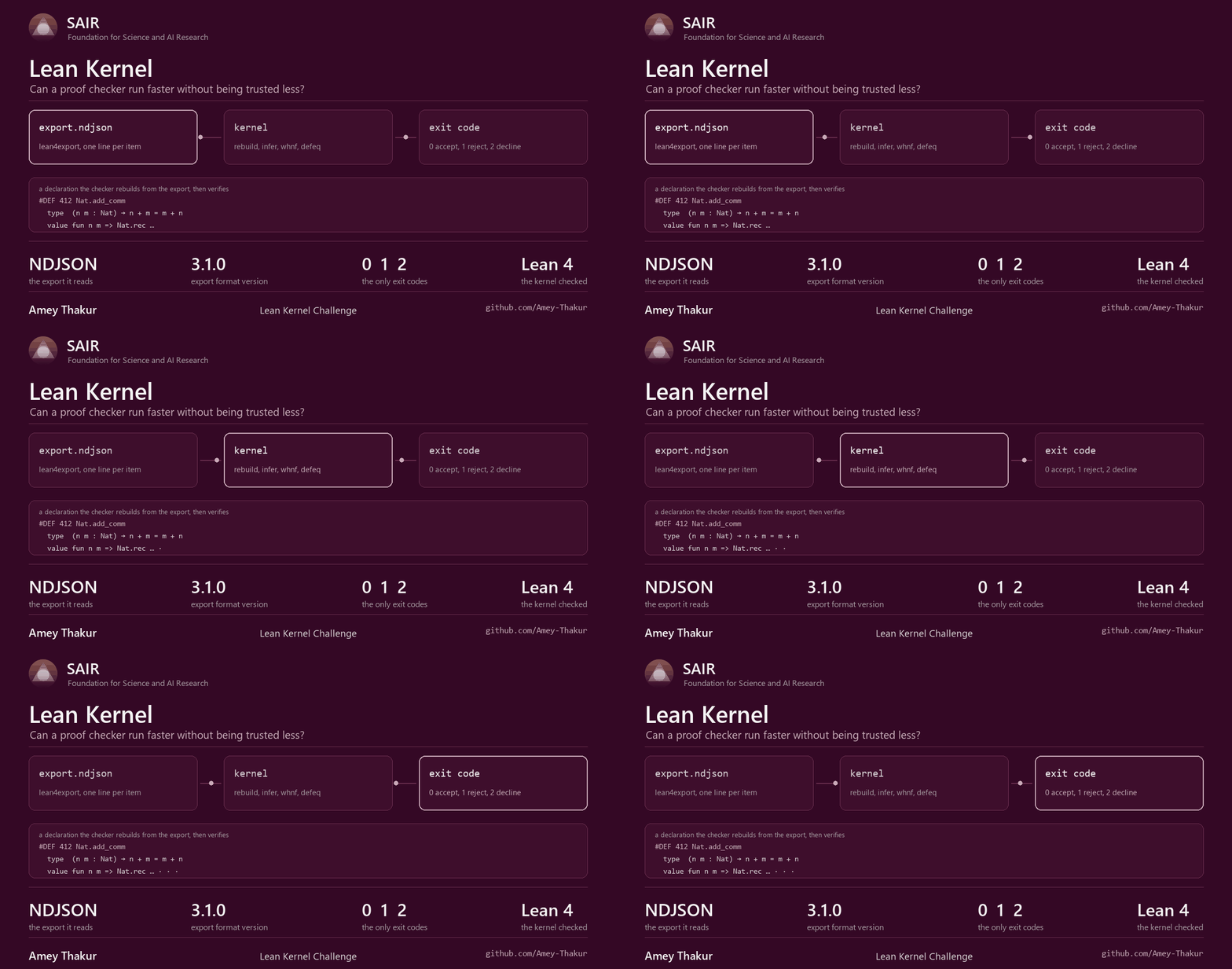
paper-data/ of
the same repository: the step model of Table 3, the timings of
Tables 4 and 5, the bound slack of
Section 4.3, the eight-problem summary, and the judge’s own figures
of Section 6.5. The same directory carries the guard that reads
this manuscript and fails if any quoted figure disagrees with those files,
which is how the two are kept from drifting apart.
Acknowledgements
The specification, the axiom rules and the test structure are the competition’s own [1]. No item from the Contributor Network and no external source was used in constructing the entry.
Citation
Please cite this work as:
Thakur, Amey. "A Whole Table Row in One Natural Number: Kernel-Checked Dynamic Programming with a Proved Width Bound" (Nov 2026). https://github.com/Amey-Thakur/SAIR-LEAN-KERNEL-CHALLENGE.Or use the BibTex citation:
@article{thakur2026leankernel,
  title   = "A Whole Table Row in One Natural Number: Kernel-Checked Dynamic Programming with a Proved Width Bound",
  author  = "Thakur, Amey",
  year    = "2026",
  month   = "Nov",
  url     = "https://github.com/Amey-Thakur/SAIR-LEAN-KERNEL-CHALLENGE"
}