Chebotarev Fingerprints: Identifying Degree-24 Galois Groups Without Computer Algebra

Abstract

Naming the Galois group of a degree-24 integer polynomial ordinarily demands resolvent computations inside a computer algebra system. This paper presents a statistical alternative that needs only polynomial factorisation modulo small primes, and evaluates it against 576,682 polynomials whose groups the SAIR IGP24 evaluation server computed independently in Magma. The method reads the multiset of Frobenius cycle types at 60 primes as a sample from the group’s own cycle-type distribution, which the Chebotarev density theorem licenses, then scores that sample against empirical profiles of candidate groups drawn by product-replacement sampling. Within its domain the classifier reaches 69.0% top-1 and 88.7% top-3 accuracy at 53 ms per polynomial. Its practical value rests on a calibrated abstention rule: required to beat the runner-up by a log-likelihood margin of 8, the classifier commits on 12.7% of inputs and answers correctly on 76 of 76 commitments, a 95% Wilson lower bound of 95.2% on precision. A separability bound explains these figures instead of merely reporting them. The Bhattacharyya coefficient between the cycle-type distributions of two groups caps the accuracy of every possible method at a given number of primes, and group theory alone computes it, before any polynomial is factored. It predicts two things and measurement confirms both: accuracy falls from 100% to 23.5% as a group’s nearest competitor closes in, respecting that cap in every band, and 60 primes is too few, since accuracy is still climbing there. Two further limitations get the same treatment. Profiles cover 24T₁ through 24T₈₀₀₀, and only 9.4% of the labelled corpus falls in that range, so coverage rather than accuracy binds deployment. Novelty counted in fingerprints overstates novelty in groups by more than an order of magnitude. All code and data are public.

Introduction

Let f ∈ ℤ[x] be monic and irreducible of degree n. Its Galois group is the automorphism group of the splitting field of f over ℚ, which acts faithfully and transitively on the n roots and therefore embeds as a transitive subgroup of S_n. Identifying that subgroup among the transitive groups of degree n, up to conjugacy, is a basic computational question in algebraic number theory. Degree 24 admits exactly 25,000 such groups, labelled 24T₁ through 24T₂₅₀₀₀; 24,193 of them are solvable and 807 are not.

The standard approach computes resolvent polynomials and inspects how they factor, descending the lattice of transitive groups. Magma, PARI/GP and Sage all implement this family of algorithms [2][3][13][9]. The approach returns an exact answer, and it costs accordingly. It also presumes that one of those systems is available.

This paper asks a narrower question. Suppose no computer algebra system is at hand, and the only available primitive is factorisation of f modulo small primes, which any integer-arithmetic library supplies. How much of the group can one recover, and how reliably? Figure 1 states the answer this paper develops as six steps and no symbols; the rest of the paper makes each step precise and measures how well it works.

The question arose in practice. Preparing submissions for the SAIR Inverse Galois Problem competition at degree 24 required deciding, before spending a submission, which group a candidate polynomial would realise, so that search effort could go toward groups no other participant had claimed. The evaluation server computes the label in Magma and returns it, but only after a submission is spent. Locally, no computer algebra system was installed. A predictor was therefore not a convenience but a precondition for directing the search at all.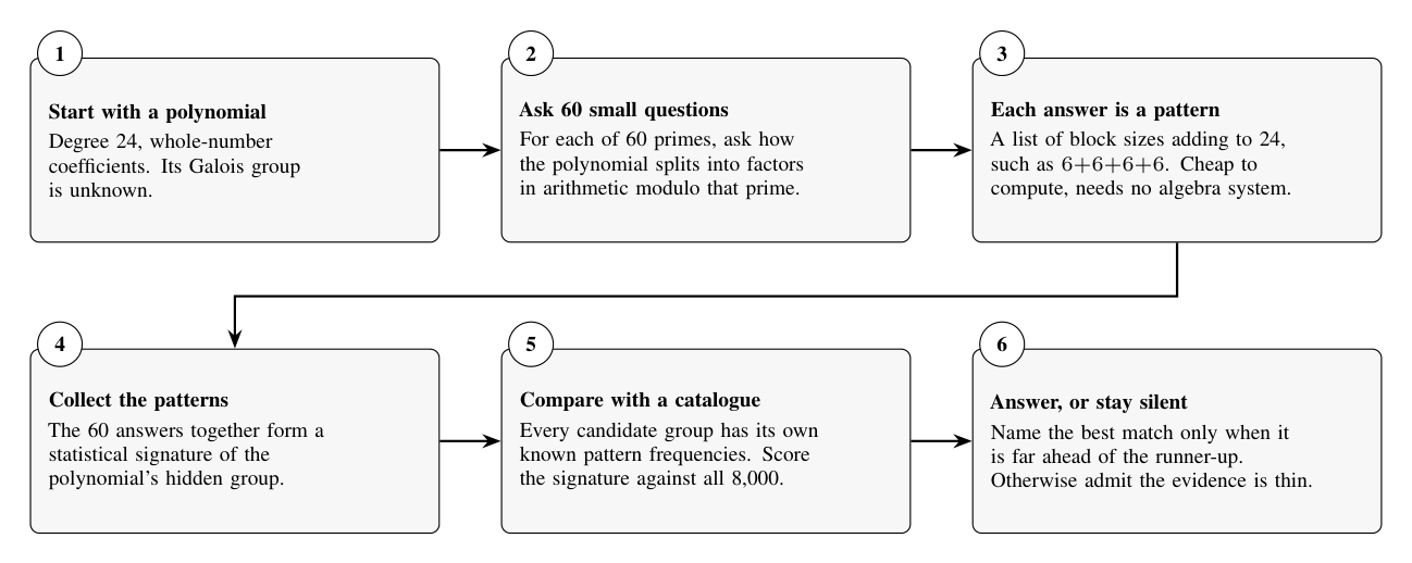

Figure 1. The method without notation. Factoring a polynomial modulo a prime is elementary arithmetic that any integer library performs, and steps 2 and 3 need nothing more. What makes the pattern informative is the Chebotarev density theorem (Section 2.2): the patterns a polynomial produces are not arbitrary but are drawn, at random, from a distribution fixed by its Galois group. Reading the observed patterns as a sample from that distribution turns identification into a statistical question. Figure 2 gives the same pipeline in the notation used throughout.

Contributions

1. A classifier that names the Galois group of a degree-24 polynomial from factorisation data alone, with no resolvent computation and no computer algebra system (Section 4).
2. An evaluation against independent ground truth. The SAIR evaluation server labelled 576,682 polynomials in Magma over the campaign. Section 7 measures the classifier against that corpus and reports 69.0% top-1 and 88.7% top-3 accuracy, each with a 95% interval.
3. A calibrated abstention rule under which the classifier answers correctly on 76 of 76 commitments while covering 12.7% of inputs (Section 4.4). For directing a search, precision without recall is the useful trade, and this rule is what made the method usable.
4. A separability bound that decides, before any polynomial is factored, which groups the method can name at all (Proposition 1). The bound predicts accuracy from the geometry of the candidate set, and Section 8 confirms the prediction: accuracy falls from 100% to 23.5% across four bands of increasing crowding, and stays under the information-theoretic ceiling in every band.
5. Two quantified negative results (Section 9). Profile coverage rather than classifier accuracy binds deployment: only 9.4% of the labelled corpus carries a true label inside the profiled range (Section 6). Separately, fingerprint novelty overstates group novelty by more than a factor of ten, which misleads any pipeline that counts its own discoveries by the statistic it uses to predict them.

Hypotheses

Four claims organise the experiments. Each one admits a measurement that could contradict it, and Section 8.4 returns to each with the evidence that bears on it.

• H1 (sufficiency). Cycle types at a few dozen primes identify a degree-24 group more often than not, within the range for which profiles exist.
• H2 (crowding binds, not evidence). The distance from a group to its nearest competitor in cycle-type distribution governs accuracy, and that distance is fixed before any polynomial is seen. Errors therefore concentrate on crowded groups rather than falling uniformly.
• H3 (calibration). The log-likelihood margin measures reliability, so thresholding it exchanges coverage for precision at a predictable rate.
• H4 (saturation). Accuracy levels off in the number of primes, so the prime budget can be fixed by measurement rather than guessed. The evidence supports H1, H2 and H3. It contradicts H4, and the contradiction is useful: the operating point this work deployed spent too few primes, and Section 8.1 measures what that cost.

Background

Frobenius elements and cycle types

Let f be as above, with splitting field K and Galois group G = Gal(K/ℚ). Let p be a prime not dividing disc(f). Reducing modulo p factors f into distinct irreducibles over 𝔽_p,

f ≡ f₁ f₂ … f_m (mod p),    deg f_i = d_i,    Σ_i=1^m d_i = n .

Dedekind's theorem states that the Frobenius automorphism at p permutes the roots of f with cycle type exactly λ(f,p) = (d₁, d₂, …, d_m), the partition of n recording those factor degrees. The theorem converts a question about a Galois group into a question about factorisation, which is the pivot the whole method turns on. ### The Chebotarev density theorem Chebotarev's theorem [[1]](#ref-1) states that Frobenius elements equidistribute across conjugacy classes: a conjugacy class C ⊆ G receives the primes whose Frobenius class is C with natural density |C|/|G|. Fix a set P of primes avoiding disc(f) and collect the observed multiset

Λ(f, P) = {  λ(f, p) : p ∈ P  } .

Chebotarev licenses reading Λ(f,P) as a sample from the cycle-type distribution of G on n points,

π_G(λ) = (|{  g ∈ G : type(g) = λ  }|)⁄(|G|) ,

a probability distribution over partitions of n.

That statement carries the entire theoretical content of the method, and it also fixes the method’s ceiling. Groups with different cycle-type distributions produce different fingerprints and separate cleanly. Groups sharing a distribution do not separate at all, however many primes one observes. Section 9 measures how often that happens.

Discriminants and signatures

The polynomial discriminant Δ(f) and the discriminant d_K of the field K = ℚ[x]/(f) satisfy

Δ(f) = d_K · i² ,

where i is the index of ℤ[x]/(f) in the ring of integers of K. The competition scores |d_K|, which PARI/GP computes through `nfdisc` [[9]](#ref-9), so a large index costs nothing provided the field discriminant stays small. The signature reduces to r, the number of real roots, which is even in even degree, so r ∈ {0, 2, …, 24}. ### The competition and its scoring rule The Inverse Galois Problem competition at degree 24 ran from 16 June to 15 August 2026 under the SAIR Foundation, which runs open competitions on unsolved problems in mathematics and computation. John Jones, Jen Paulhus, David Roe, Andrew Sutherland and Terence Tao co-organised it in collaboration with the LMFDB [[6]](#ref-6)[[7]](#ref-7). The arrangement matters for this paper beyond provenance: the same project that supplies the baseline of Section 2.4 and the generators of Section 4.2 also defines the target the classifier is measured against, so the labels, the candidate set and the notion of novelty all come from one consistent source.

The competition [6] scores each distinct pair (24T_t, r). Writing k for the number of teams holding a pair, D for the submitter’s best absolute field discriminant and D₀ for the smallest any team achieved,

points = 2^1-k · (log D₀)⁄(log D) .

(1)

The exponential factor dominates. Ten teams holding a pair reduce its value to 2^-9 of a pair held alone, so whether anyone else found the same group governs the value of a submission, while the quality of the discriminant contributes only logarithmically. Of the 165,836 possible (24T_t, r) pairs, the frozen LMFDB baseline [[7]](#ref-7) covered 286 labels and 622 pairs, under half of one percent. That sparsity is what made the space worth searching. It is also what made blind search unrewarding, because dense random polynomials fall into 24T₂₅₀₀₀ = S₂₄ and into A₂₄, which every participant already holds.

Equation (1) explains why this work needed a predictor rather than merely benefiting from one. Without one, a search yields polynomials whose value stays unknown until a submission has already been spent on them.

Related work

**Exact determination of Galois groups.**Stauduhar [2] introduced the relative resolvent method, which descends the lattice of transitive groups and tests resolvents for rational roots. Fieker and Klüners [3] extended the approach to higher degrees with practical algorithms that underpin current computer algebra implementations. These methods return certainties. The present method returns evidence, and the two therefore answer different questions: a resolvent computation proves a group, whereas a fingerprint ranks candidates cheaply enough to steer a search of hundreds of thousands of polynomials. **Factorisation patterns as group evidence.**Constraining a Galois group by its factorisation pattern is standard for small degrees, where a handful of primes often eliminates all but one candidate. Degree 24 changes the character of the problem. With 25,000 candidate groups, elimination fails and the task becomes statistical discrimination among thousands of similar distributions. This paper treats it explicitly as maximum-likelihood classification over sampled distributions, and measures it with the vocabulary of classification: accuracy, precision, coverage and abstention. **The Inverse Galois Problem.**Whether every finite group arises as a Galois group over ℚ remains open. Malle and Matzat [4] and Serre [5] collect the rigidity, specialisation and embedding-problem techniques that settle large families. The competition inverts the usual emphasis. Rather than realising one prescribed group, participants search broadly and must then identify what they have produced, which moves identification, not construction, into the critical path. **Sampling finite groups.**Celler et al. [8] introduced product replacement, a random walk that generates near-uniform elements of a finite group from a generating set. Section 4.2 uses it to estimate π_G for candidate groups, taking generators from the LMFDB [7]. **Positioning within the author’s prior work.**Three strands of the author’s earlier work bear directly on the design adopted here. The accident-detection pipeline of Thakur and Talele [15] assigns labels zero-shot, without training on examples of the target classes. The classifier below does the same: its profiles come from group theory and never from labelled polynomials, so no polynomial in Table 4 could have leaked into training. The gesture detector of Thakur [16] identifies a class from a deterministic structural signature, the projected winding order, rather than from a learned representation; Section 4 follows that pattern and substitutes the cycle-type multiset as the signature. The treatment of graded confidence in Thakur et al. [17] motivates the decision rule of Section 4.4, which acts above a confidence threshold and withholds judgement below it, the trade Table 4 quantifies. The maximum-likelihood framing and the vocabulary of decision rules follow the classification treatment in Thakur and Konde [18]. **Crowding rules in open scientific competitions.**The exponential factor of Equation (1) recurs across SAIR competitions. A companion study of the Andrews-Curtis Challenge under the same 2^1-k rule [19] finds that solver competence and point value are anti-correlated by construction, because a target is widely shared precisely when it is easy to reach. Section 10 reports the same mechanism operating here, which suggests the effect belongs to the scoring rule rather than to either problem.

Method

Figure 2 shows the pipeline. A polynomial enters, factorisation modulo a fixed prime set produces its fingerprint, and the fingerprint is scored against precomputed group profiles to yield either a committed label or an abstention.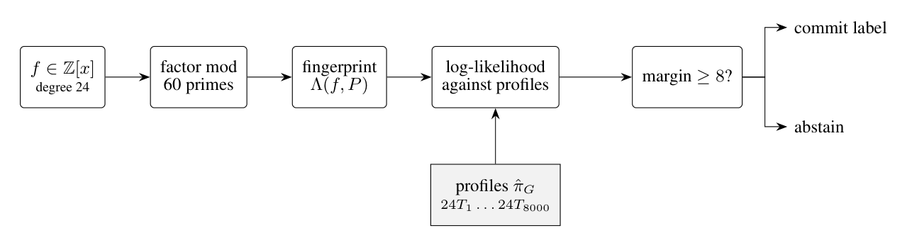

Figure 2. The classifier. Factorisation supplies the only evidence; the profiles depend on group-theoretic data alone and never on the polynomial under test.

Fingerprints

Definition 1 (Fingerprint). Fix a set P of primes. The fingerprint of f is the multiset Λ(f, P) of cycle types λ(f,p) taken over those p ∈ P at which f stays squarefree modulo p. The implementation uses two prime sets, listed in Table 1. Clustering needs only to decide whether two polynomials plausibly share a group, and 24 primes suffice. Classification must name one group among thousands, which demands more resolution, so it uses 60. Both remain inexpensive: factoring a degree-24 polynomial modulo a small prime costs on the order of a millisecond through python-flint.

Purpose	Primes	Count
Clustering, deduplication	101, 103, …, 227	24
Classification	101, 103, …, 439	60

Table 1. Prime sets. All lie above the coefficient range of the generated families, which keeps ramified primes rare.

Group profiles

For each candidate group G the pipeline estimates a profile π̂_G by walking the group with product replacement [8] from generators supplied by the LMFDB [7], recording the cycle type of each sampled element and normalising the counts. Profiles exist for 24T₁ through 24T₈₀₀₀, which Section 9.1 identifies as the binding constraint on the method as deployed.

The classifier

Given an observation Λ(f,P) and the profiles, the classifier assigns each group the log-likelihood

ℓ(G) = Σ_{λ ∈ Λ(f,P)} log max(π̂_G(λ),  ε),    ε = 10^-4,

(2)

and predicts argmax_G ℓ(G).

The floor ε does real work. A profile is a finite sample, so a cycle type genuinely attainable in G can be missing from π̂_G by chance. Scoring that absence as log 0 = -∞ would eliminate the true group on a single unlucky observation. Replacing it with a large finite penalty preserves the ranking while keeping the true group recoverable, which turns a brittle rule into a usable one.

Prime p	Cycle type of f mod p
101	142244
103	2444
107	14210
109	2444
113	64
127	64
… and 54 more primes

Rank	Candidate	ℓ(G)
1	24T7142 (true group)	-124.8
2	24T4860	-135.2
3	24T4806	-136.1

Table 2. The method on one polynomial. Each prime contributes the cycle type of its factorisation, shown left as a partition of 24 in exponent notation, so 1⁴2²4⁴ means four linear factors, two quadratic and four quartic. Summing Equation (2) over all 60 observations ranks the candidates, shown right. The leader beats the runner-up by 10.4, above the margin of 8, so the classifier commits, and it is correct. The gap is the whole decision: the ranking alone would be the same whether the evidence were decisive or not.

Abstention

A confident error costs more than silence. It sends search effort toward a group the polynomial will not realise, and that effort is unrecoverable. The classifier therefore commits only when the evidence separates the leader decisively.

Definition 2 (Confident prediction). Let ℓ₍₁₎ ≥ ℓ₍₂₎ denote the two largest log-likelihoods and let τ > 0 be a margin. The classifier commits to the leading label when ℓ₍₁₎ - ℓ₍₂₎ ≥ τ, and abstains otherwise. Table 2 follows one polynomial through the whole procedure, from its factorisations to the ranked candidates and the margin that decides whether the classifier speaks.

A margin in log-likelihood is a likelihood ratio. Setting τ = 8 requires the leading group to explain the observed factorisation data at least e⁸ ≈ 2981 times better than its nearest rival. Every result below uses τ = 8.

Separability: what the evidence can decide

Accuracy is usually treated as a property of a classifier. Much of it here is a property of the problem. Two groups whose elements have the same distribution of cycle types cannot be told apart by factorisation at any number of primes, and two groups whose distributions are merely close need proportionally more primes to separate. This section makes that quantitative, which gives the experiments something to predict rather than merely describe.

A coefficient that bounds every decision rule

Write 𝒯 for the set of cycle types available in degree 24; 231 of them occur across the 8,000 profiles. This is the alphabet the observations are drawn from, not the multiset Λ(f,P) observed for a particular polynomial. For a transitive G ≤ S₂₄ let π_G be its cycle-type distribution, so π_G(λ) is the proportion of elements of G with cycle type λ. For two groups define the Bhattacharyya coefficient

ρ(G,H) = Σ_{λ ∈ 𝒯} √π_G(λ) π_H(λ) ∈ [0,1].

It equals 1 exactly when π_G = π_H and 0 when the two groups share no cycle type. Table 3 shows a pair at ρ = 0.99, which makes the abstraction concrete: two groups placing almost the same mass on the same handful of cycle types. Bhattacharyya [[10]](#ref-10) introduced it as a measure of divergence between populations; it is the Hellinger affinity of the two distributions [[12]](#ref-12), and it multiplies over independent observations, which is what makes it the right currency for counting primes. | Cycle type λ | π_G(λ) | π_H(λ) | √π_G π_H | |---|---:|---:|---:| | 6⁴ | 0.2433 | 0.2447 | 0.2440 | | 12² | 0.1747 | 0.1693 | 0.1720 | | 3⁴6² | 0.1557 | 0.1717 | 0.1635 | | 3⁸ | 0.0857 | 0.0793 | 0.0824 | | 1⁴2⁶4² | 0.0837 | 0.0623 | 0.0722 | | 2⁴4⁴ | 0.0670 | 0.0763 | 0.0715 | | all 16 types with mass | ρ = 0.9900 | | |

Table 3. Why a coefficient near 1 is fatal. G = 24T₃₈₆₀ and H = 24T₃₇₈₉ place almost the same mass on the same cycle types, so a factorisation drawn from either looks the same. The right-hand column sums to ρ = 0.9900, and Proposition 1(ii) then forbids any method from separating them at 60 primes with error below 8%. No amount of classifier design recovers this; only more primes do.

Proposition 1. Let G and H be equally likely a priori, and let λ₁,…,λ_m be the cycle types of f at m primes unramified in both, modelled as independent draws from π_G or from π_H. Write ρ = ρ(G,H). Then

1. the likelihood-ratio test decides wrongly with probability at most 1⁄2ρ^m, and

2. every rule that sees only λ₁,…,λ_m decides wrongly with probability at least 1⁄2(1 - √1 - ρ^2m).

Proof. Under the model the two hypotheses are the product measures p = π_G^{⊗ m} and q = π_H^{⊗ m}. The coefficient multiplies over products, so ρ(p,q) = ρ^m.

Under a uniform prior the least error any rule attains is the Bayes error 1⁄2Σ_x min(p(x),q(x)), achieved by the likelihood-ratio test. For (i), min(a,b) ≤ √ab for non-negative a and b, so the Bayes error is at most 1⁄2Σ_x √p(x)q(x) = 1⁄2ρ^m.

For (ii), the Bayes error equals 1⁄2(1 - ‖ p - q ‖_TV). Let h²(p,q) = Σ_x (√p(x) - √q(x))² = 2(1 - ρ(p,q)) be the squared Hellinger distance, written h rather than H because H already denotes a group here. The standard comparison ‖ p - q ‖_TV ≤ h√1 - h²/4 [12] becomes, after substituting h² = 2(1-ρ(p,q)),

‖ p - q ‖_TV ≤ √1 - ρ(p,q)² = √1 - ρ^2m .

Since no rule beats the Bayes error, every rule errs with probability at least 1⁄2(1 - √1-ρ^2m). □ The two halves do different work, and conflating them is the easiest mistake to make with a bound of this kind. Part (i) states when success is guaranteed and says nothing otherwise, so a pair it fails to cover may still be classified correctly. Part (ii) forbids: a group whose nearest competitor sits at ρ cannot be named more reliably than the stated figure, whatever classifier is used and however the evidence is weighed. The negative result in Section 8 rests on (ii) alone.

Corollary 2. To hold the pairwise error below δ < 1⁄2 it suffices to use

m ≥ (log(1/2δ))⁄(log(1/ρ))

primes. Against N candidate groups rather than two, a union bound over the N-1 competitors replaces δ by δ/(N-1), so the requirement grows only as log N: multiplying the size of the candidate set by ten costs a fixed number of additional primes, not a fixed factor.

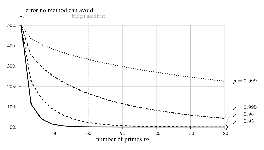
Figure 3. The bound of Proposition 1(ii): the smallest error any method can achieve when a group's nearest competitor sits at coefficient ρ. The vertical line marks the 60 primes this work spent. At ρ=0.95 that budget is ample, at the measured median of 0.98 it is adequate, and beyond 0.995 it leaves an error floor no classifier can remove. Section 5.2 gives the measured distribution of ρ, and Table 6 the accuracy that results.

What the bound predicts here

For a group G the binding quantity is its nearest competitor anywhere in the profile set,

ρ^*(G) = max_{H ≠ G} ρ(G,H),

computed once from the profiles alone and independent of any polynomial. Across the 8,000 profiles, ρ^* has median 0.9805, ninetieth percentile 0.9984 and maximum 0.9999. Figure 4 gives the whole distribution. The candidate set is crowded: for a typical group some other group produces almost the same factorisation statistics, and only 4.9% of groups have a competitor further away than ρ = 0.9.

Corollary 2 converts this into a prime count. Driving the pairwise error below 5% against the nearest competitor takes a median of 117 primes, so the 60 the classifier uses guarantee that error rate for only 31.0% of groups. Applying the union bound over all 7,999 competitors raises the median requirement to 573 primes. Two predictions follow, and Section 8 tests both.

1. Accuracy should fall as ρ^* rises, and should stay below the ceiling 1 - 1⁄2(1-√1-ρ^*2m) that part (ii) imposes at m = 60.
2. Accuracy should not yet have saturated at 60 primes, since the budget falls well short of what the sufficiency direction asks for.

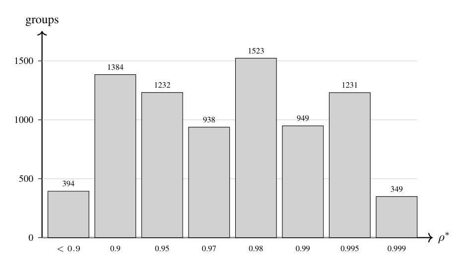
Figure 4. Nearest-competitor distance across the 8,000 profiled groups, by lower edge of each band. Only 394 groups, 4.9% of the set, have a competitor further than ρ = 0.9; most sit above 0.95. The candidate set is crowded almost everywhere, which is what Figure 3 converts into an error floor.

What the model idealises

Two idealisations enter, and both work against the bound’s reliability rather than for it.

Chebotarev is an asymptotic statement. It gives the density of primes whose Frobenius class lies in a given conjugacy class, not independence across a fixed finite set of 60 small primes. Treating the observations as independent draws is an approximation, and Proposition 1 inherits it. Effective forms of the theorem exist [11], but their error terms are governed by the discriminant of the splitting field, which for a degree-24 field is far too large for a bound at 60 primes near 100 to say anything useful. The approximation is therefore not one this paper can discharge by citing a sharper theorem, which is why it is tested empirically instead. The approximation is the same one the classifier itself makes, so the bound and the method stand or fall together, which is why the empirical test in Section 8 carries the weight.

Second, π_G is not known exactly. The profiles estimate it from 3,000 product-replacement samples for each group, so ρ is itself an estimate. Sampling noise biases that estimate downward where two distributions are genuinely close, because two finite samples drawn from one distribution do not give ρ = 1. The separability figures above are therefore optimistic at the hard end, and the true crowding is at least as severe as reported.

Experimental setup

**Ground truth.**The SAIR evaluation server computes the 24T_t label of each submitted polynomial in Magma [13] and returns it with the verification response. The campaign accumulated 576,682 labelled polynomials spanning 3,995 distinct labels. This ground truth is unusually strong for a study of this kind. The labels come from a different method, resolvent computation rather than statistics; from a different implementation, which the author never ran and could not inspect; and from a party with no stake in the classifier’s performance, namely the competition organisers [6]. Nothing in the evaluation depends on the author’s own judgement of what a polynomial’s group is, which is the usual weak point in a study that proposes a classifier and then measures it. **Domain of evaluation.**The classifier can name only a group it holds a profile for. Among the labelled polynomials, 54,350, or 9.4%, carry a true label inside the profiled range. Drawing an evaluation sample uniformly from the corpus would therefore cap measured accuracy near 9.4% however well the method discriminates, reporting profile coverage under the name of predictive power. This paper separates the two: Section 7 measures accuracy inside the domain, and Section 9.1 reports coverage as the distinct limitation it is. **Protocol.**From the in-domain polynomials the evaluation drew 600 uniformly at random under a fixed seed. No evaluation polynomial influenced any profile, since profiles derive from group-theoretic data alone.

Results

Measure	Value	95% interval
Top-1 accuracy	414 / 600 = 69.0%	[65.2%, 72.6%]
Top-3 accuracy	532 / 600 = 88.7%	[85.9%, 91.0%]
Confident commitments	76 / 600 = 12.7%
Confident precision	76 / 76 = 100%	≥ 95.2%
Abstentions	524 / 600 = 87.3%
Time per polynomial, reference	409 ms
Time per polynomial, vectorised	53 ms

Table 4. Classifier performance on 600 polynomials drawn from the in-domain portion of the server-labelled corpus, at margin τ = 8. Intervals are Wilson score intervals [[14]](#ref-14). The two timings run the same classifier and return the same rankings; the campaign used the reference implementation, and Section 8.3 explains the difference.

Table 4 reports the measurement, and three points follow from it. **The classifier ranks well even when it does not lead correctly.**Top-1 accuracy reaches 69.0% and top-3 reaches 88.7%. The gap shows that failures are usually failures of separation rather than of candidacy: the true group sits among the leaders but does not pull clear of them. Groups with similar cycle-type distributions produce exactly this signature, which is what Section 7.1 predicts and what motivates abstention. **Confident mode made no errors on this sample.**The classifier committed 76 times and was right 76 times. A point estimate of 1 says little on its own, so the honest summary is an interval. For x = n successes in n trials the Wilson score lower bound [[14]](#ref-14) collapses to

(n)⁄(n + z²) = (76)⁄(76 + 1.96²) = (76)⁄(79.84) = 0.952 ,

(3)

so the data support precision of at least 95.2% at the 95% level. The claim this paper makes is "no errors in 76 commitments, precision at least 95.2%", not an unqualified 100%. **The method trades recall for precision by design.**The classifier abstains on 87.3% of inputs. A general-purpose identification tool operating there would be close to useless. A targeting tool operating there is well placed, because an abstention costs only that the pipeline treats the polynomial as unknown and explores it anyway, while a confident error costs search effort spent against a group that will never appear. ### Why similar groups bound the method The ceiling is structural, not an artefact of sample size. Two groups sharing a cycle-type distribution are indistinguishable to any amount of factorisation evidence, because Equation (2) reads only that distribution. More primes sharpen the estimate of which distribution generated the data; they cannot separate two groups that induce the same one. Raising top-1 accuracy beyond a certain point therefore requires evidence outside factorisation patterns, such as a resolvent, and not merely a longer prime list. ### Choice of margin The margin τ slides the operating point along a precision-recall curve without altering the classifier. Lowering τ buys coverage and admits errors; raising it does the reverse. This work fixed τ = 8 during the campaign, on a different sample, and reports it here unchanged rather than tuning it to the evaluation. ## Analysis Section 7 reports what the classifier does. This section asks why, along the three axes the hypotheses of Section 1.2 name: how much evidence the method needs, where its mistakes fall (Section 8.2), and whether the separability bound of Section 5 describes the behaviour observed. All three experiments run on the same 600 in-domain polynomials at the same margin, and the script that produces them, `scripts/analysis.py`, is in the repository.

Scoring 8,000 candidate groups for every prefix of the prime list would be prohibitive one group at a time, so the analysis scores all groups at once as a matrix product. That reimplementation earns its place only if it agrees with the released predictor, and it does: on 25 polynomials the two rank candidates identically, and at 60 primes the matrix scorer reproduces the accuracy, top-3 rate and coverage of Table 4 exactly. The experiments below therefore measure the classifier this paper reports, not a variant of it.

How many primes the classifier needs

Factorisation dominates the cost, so the prime count is the parameter worth tuning. Because the log-likelihood is a sum over observations, scores at m primes are a prefix of the scores at 60, and a single factorisation pass yields every row of Table 5.

Primes	Top-1	Top-3	Coverage	Confident precision
5	7.0%	14.8%	0.0%	no commitments
10	19.8%	32.7%	0.3%	2 of 2
15	29.7%	48.0%	0.7%	4 of 4
20	39.5%	58.2%	1.5%	9 of 9
30	50.0%	72.7%	3.7%	22 of 22
40	61.5%	82.0%	6.8%	41 of 41
50	64.0%	84.5%	9.0%	54 of 54
60	69.0%	88.7%	12.7%	76 of 76

Table 5. Accuracy against the number of primes, on the same 600 in-domain polynomials. The final row is the operating point of Table 4. Accuracy is still climbing at the right-hand edge, and confident precision holds at every budget.

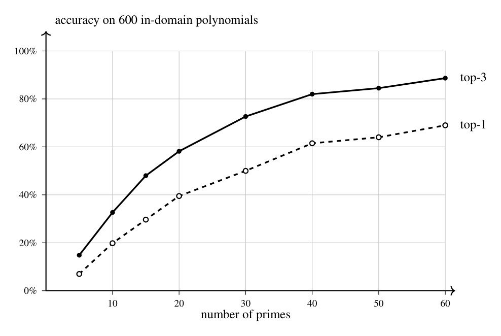
Figure 5. Accuracy against prime count. Neither curve has flattened at 60 primes, the budget this work deployed, so the operating point sits on the rising part of the curve rather than at a saturation point.

Two findings follow. First, accuracy has not saturated. The last ten primes add 5.0 points of top-1 accuracy and 4.2 of top-3, and raise confident coverage from 9.0% to 12.7%. Figure 5 shows both curves still rising at the right-hand edge. H4 is therefore false as stated: 60 primes was a budget, not a measured optimum, and the measurement says the budget was set too low. This matches the second prediction of Section 5.2, which put the median requirement near 117 primes. The cost of correcting it is mild, since factorisation at one more prime costs under a millisecond, and Section 8.3 gives the arithmetic.

Second, confident precision holds at 100% at every budget, across commitments ranging from 2 to 76. The margin rule is not tuned to the operating point; it survives a twelvefold change in the evidence available to it. This is the clearest support for H3, and it is stronger evidence than the single operating-point figure in Table 4, which a favourable sample could produce by chance.

Where the mistakes fall

Section 5.2 predicts that accuracy tracks ρ, the coefficient between a group and its nearest competitor. Because ρ depends only on the profiles, it is fixed before any polynomial is examined, so grouping the test set by it tests a prediction rather than describing an outcome.

Nearest competitor ρ*	Polynomials	Top-1 accuracy	Ceiling
below 0.95	75	100.0% (95.1–100.0)	100.0%
0.95 to 0.99	335	81.2% (76.7–85.0)	99.3%
0.99 to 0.999	156	37.8% (30.6–45.6)	84.8%
0.999 and above	34	23.5% (12.4–40.0)	62.1%

Table 6. Accuracy against the crowding of the true group's neighbourhood, with 95% Wilson intervals. The ceiling is the largest accuracy Proposition 1(ii) permits any method at 60 primes, evaluated at the midpoint of each band. Accuracy falls monotonically as crowding rises and respects the ceiling in every band.

Table 6 confirms the prediction. Accuracy falls from 100.0% to 23.5% across the four bands, monotonically, and in no band does it exceed the ceiling that Proposition 1(ii) allows. Where the theory says the problem is easy, in the 75 polynomials whose groups have a distant nearest competitor, the classifier makes no mistakes at all. Where the theory says the problem is nearly undecidable at 60 primes, accuracy collapses. The evidence supports H2.

The gap between the measured accuracy and the ceiling widens as crowding increases, from nothing in the first band to 47 points in the third. Two readings are available and the data here does not separate them. The bound may be loose, since the Bhattacharyya inequality is not tight; or the classifier may lose ground to the true optimum exactly where discrimination is hardest. The ceiling is also a pairwise quantity applied to an 8,000-way problem, which makes it conservative as an upper bound on accuracy. What the table establishes is the direction and the ordering, not the size of the gap.

A second, weaker comparison points the same way. Taking each polynomial’s strongest rival, the highest-ranked group other than the true one, the median coefficient between truth and rival is 0.9684 when the classifier is right and 0.9867 when it is wrong. Comparing the true group with the predicted group instead would be vacuous, since a correct prediction names the true group and scores 1 by construction. This comparison carries a confound the bands in Table 6 do not: the rival is the runner-up when the classifier is right and the leader when it is wrong, so the two cases sit at different ranks. This comparison corroborates Table 6; it does not carry the argument.

When the classifier is wrong it is rarely far wrong. The true label has median rank 3 among 8,000 candidates and lies within the top ten for 91.4% of errors. The failure is one of discrimination among near-identical candidates, not of misdirection, which is what Table 6 would lead one to expect and what makes the top-3 figure and the abstention rule useful.

Cost

The reference implementation scores one candidate group at a time and runs at 409 ms per polynomial. Scoring all 8,000 groups as a single matrix product leaves every ranking unchanged and brings this to roughly 53 ms, of which 35 ms is factorisation and 17 ms scoring. That 17 ms covers the eight prefixes of Table 5 rather than a single prediction, so it overstates the cost of one call.

The consequence matters more than the speedup. Once the scorer handles all groups at once, factorisation dominates, and factorisation costs roughly 0.6 ms per prime, linear in the budget. Buying the 57 extra primes that Section 5.2 asks for would cost about 35 ms per polynomial, less than the saving just described. The budget that Table 5 shows to be too low can be corrected without exceeding the cost of the implementation this work actually deployed.

The hypotheses

H1 holds: 69.0% top-1 accuracy inside the profiled range, against a candidate set of 8,000 and with no computer algebra system, exceeds the more-often-than-not threshold with a 95% interval of 65.2% to 72.6%.

H2 holds. Accuracy falls monotonically across four bands of increasing crowding, a quantity fixed before any polynomial is seen, and respects the information-theoretic ceiling in each band.

H3 holds, and more strongly than the operating point alone shows. Confident precision is 100% at every one of eight prime budgets, across 2 to 76 commitments.

H4 fails. Accuracy is still rising at 60 primes, so the deployed budget was too small. The separability analysis predicted this before the ablation was run, and Section 8.3 shows the correction is affordable. Reporting the prediction and the refutation together is the point: the bound earns confidence by forecasting a result that contradicted the design in use.

Limitations

Three limitations bound what the method can claim, and Section 9.4 collects the threats to the validity of the measurements themselves.

Coverage binds before accuracy does

The dominant practical constraint is silence, not error. Profiles cover 8,000 of the 25,000 groups, and the labelled corpus concentrates outside that range: 90.6% of labelled polynomials realise a group the classifier holds no profile for. Table 7 sets the two limits side by side. Extending coverage is a matter of computation rather than research, and it is the single highest-value improvement available to this method.

	Count	Share
Transitive groups of degree 24	25,000
with a sampled profile	8,000	32.0%
Server-labelled polynomials	576,682
whose true label has a profile	54,350	9.4%
outside the profiled range	522,332	90.6%
Distinct labels observed in the corpus	3,995

Table 7. Coverage, which bounds deployment more tightly than accuracy does. A uniform sample of the corpus would cap measured top-1 accuracy at 9.4%.

Fingerprint novelty overstates group novelty

A fingerprint is a statistic, not a separating invariant. Distinct groups can share a cycle-type distribution, and in this data many do, so the map from fingerprints to labels is many-to-one in the direction that matters. Joining the campaign ledger to the server’s labels shows the consequence: roughly 10,000 fingerprint clusters that the pipeline judged novel collapsed to roughly 771 genuinely new (24T_t, r) pairs, an overstatement exceeding an order of magnitude.

The methodological lesson generalises beyond this competition. A search pipeline that counts distinct fingerprints as distinct discoveries will report progress it has not made. Novelty has to be measured against labels, never against the statistic used to predict them.

Evidence, not proof

A confident prediction is evidence. Chebotarev guarantees equidistribution in the limit, 60 primes form a finite sample, and the floor ε in Equation (2) softens the likelihood further. The method suits search direction and does not suit any setting that requires a certificate. Where certainty matters, a resolvent computation remains necessary.

Threats to validity

Four threats bear on the conclusions above.

Sample size. Every accuracy figure rests on 600 in-domain polynomials. The Wilson intervals quantify this, and the narrowest conclusions, such as the ordering in Table 6, survive comfortably. The 34 polynomials in the most crowded band give an interval from 12.4% to 40.0%, wide enough that the value of that band should be read as an order of magnitude.

Corpus composition. The evaluation corpus is what the campaign submitted, not a uniform sample of degree-24 polynomials. Submissions favoured groups the search targeted, so the distribution of true labels is not the natural one. The in-domain restriction removes the largest distortion but not this one, and the accuracy reported here describes performance on polynomials of the kind this campaign generated.

Profile estimation. Profiles rest on 3,000 product-replacement samples per group. Product-replacement approximates uniform sampling without guaranteeing it at a fixed number of steps, so a systematic bias in the sampler would propagate to every profile. Section 5.3 notes the direction of the resulting error in ρ.

Independence. Proposition 1 and the classifier both treat cycle types at distinct primes as independent draws. Chebotarev licenses this asymptotically, not at 60 fixed small primes. The empirical agreement in Table 6 is evidence that the approximation holds well enough to be useful here; it is not a proof that it holds, a distinction Section 9.3 draws out.

Application and outcome

The campaign used the classifier to steer submission batches toward groups that the competition’s intelligence endpoints reported as unclaimed or weakly held, following Equation (1). Fingerprint-based deduplication kept batches distinct, and the ledger recorded 610,718 clusters across the campaign.

The final standing was rank 54 of 256 teams, scoring 2.3559 across 10,180 scoreable pairs. The distance between a five-figure count of scoreable pairs and a score near two is entirely the exponential factor of Equation (1): the pairs obtained were, in the main, pairs other teams also held. This is the empirical shape of the same effect the companion Andrews-Curtis study reports under the identical rule [19]. Volume proved achievable and rarity did not, and only rarity pays.

Conclusion

Factorisation data alone identifies the Galois group of a degree-24 polynomial often enough to be useful, and under a calibrated abstention rule reliably enough to act on. The measured operating point is 69.0% top-1 accuracy, 88.7% top-3, and no errors across 76 confident commitments, a precision of at least 95.2% at 95% confidence, obtained in 53 ms per polynomial without a computer algebra system.

What distinguishes this account from a report of measurements is that the measurements were predicted. Proposition 1 turns the geometry of the candidate set into a ceiling on the accuracy of any method whatsoever, and that ceiling is computable from group theory before a single polynomial is factored. It called both results correctly: accuracy tracks the crowding of a group’s neighbourhood, falling from 100% to 23.5% across four bands while staying under the ceiling in each, and the 60-prime budget this work deployed is too small, a verdict the ablation then confirmed. A bound that contradicts the design in use, and turns out to be right, has earned more trust than one that ratifies it.

The limitations carry as much information as the result. Coverage, not accuracy, prevents deployment at scale, and computation alone would remedy it. Fingerprint novelty overstates group novelty by more than an order of magnitude, which traps any search pipeline that measures its own progress by the statistic it uses to predict labels rather than by the labels themselves. The honest summary is that the method works where the mathematics says it can, fails where the mathematics says it must, and now carries the means to tell the two cases apart in advance. Section 11 lists the scripts that regenerate every table above.

Data and code availability

All code and data live at https://github.com/Amey-Thakur/SAIR-INVERSE-GALOIS-PROBLEM-IGP24 [20]. The classifier is scripts/predict_label.py and the fingerprint routine is scripts/fingerprint.py. Two scripts regenerate the tables: scripts/evaluate_predictor.py reproduces Table 4, and scripts/analysis.py reproduces Tables 5 and 6 together with the separability figures of Section 5.2, writing its output as JSON. The directory data/ holds the group profiles, the server-labelled corpus and the submission ledger.

The evaluation sample is drawn under a fixed seed, so the 600 polynomials behind every table are the same 600 on any machine. Reproducing the paper needs Python 3.10 or later, python-flint for factorisation and NumPy. It needs no computer algebra system, which is the point of the method.

---

Citation

Please cite this work as:

Thakur, Amey. "Chebotarev Fingerprints: Identifying Degree-24 Galois Groups Without Computer Algebra" (Sep 2026). https://github.com/Amey-Thakur/SAIR-INVERSE-GALOIS-PROBLEM-IGP24.

Or use the BibTex citation:

@article{thakur2026chebotarev,
  title   = "Chebotarev Fingerprints: Identifying Degree-24 Galois Groups Without Computer Algebra",
  author  = "Thakur, Amey",
  year    = "2026",
  month   = "Sep",
  url     = "https://github.com/Amey-Thakur/SAIR-INVERSE-GALOIS-PROBLEM-IGP24"
}

---

References