This study examines regression analysis within Supervised Machine Learning, focusing on Simple Linear Regression (SLR) and Multiple Linear Regression (MLR). A practical implementation demonstrates the predictive relationship between study hours and grades.
Introduction
Machine Learning enables computational systems to identify patterns and generate predictions from data. Supervised Learning, a core paradigm, relies on labeled datasets to train models, with primary tasks including Classification and Regression.
Regression predicts continuous numerical outcomes by modeling relationships between dependent and independent variables. Simple Linear Regression captures the effect of a single predictor, while Multiple Linear Regression incorporates multiple predictors, providing a more detailed representation of complex relationships.
This discussion explores the theoretical foundations of SLR and MLR, the supervised learning workflow, and the statistical assumptions and evaluation metrics, including R-squared and p-values. Implementation examples illustrate both SLR and MLR, including a 3D visualization of MLR convergence. The relevance of regression analysis is further highlighted through applications in finance, healthcare, and marketing.
Hierarchy of Machine Learning Algorithms
Machine learning algorithms are generally categorized according to their learning style. The primary paradigms include Supervised Learning, Unsupervised Learning, and Reinforcement Learning.
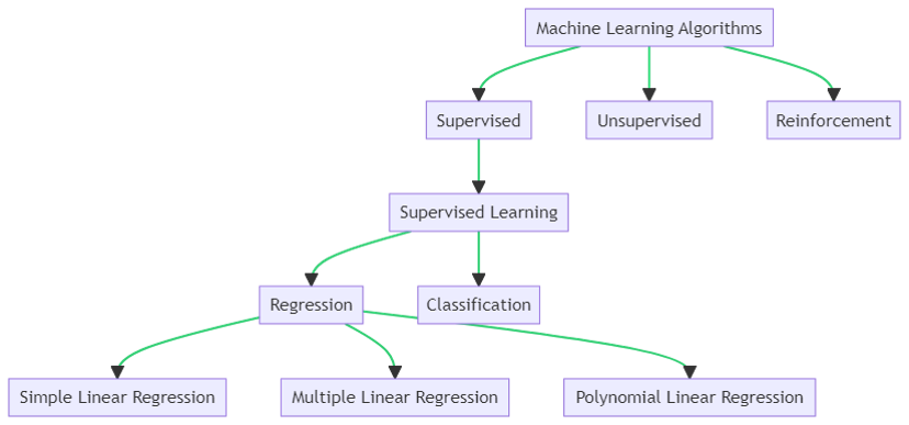
Hierarchy of Machine Learning Algorithms
Supervised Learning
This paradigm relies on labeled datasets, where the “correct” answers are known, to train algorithms to make accurate predictions or classifications. Within supervised learning, tasks are typically divided into Regression and Classification. Regression focuses on predicting continuous outcomes, while classification addresses discrete categories.
Unsupervised Learning
In unsupervised learning, algorithms analyze unlabeled data to identify hidden patterns, structures, or groupings without prior guidance.
Reinforcement Learning
Reinforcement learning trains algorithms to make a sequence of decisions through trial-and-error interactions with an environment, receiving feedback in the form of rewards or penalties.
Since this study concentrates on predicting continuous variables, such as grades based on study hours, the scope is restricted to the Regression branch of Supervised Learning. Regression techniques can be further classified as:
- Simple Linear Regression (SLR): Models the relationship between one dependent variable and a single independent variable.
- Multiple Linear Regression (MLR): Extends SLR to include multiple independent variables, enabling more complex predictive modeling.
- Polynomial Regression: Captures non-linear relationships between variables through polynomial transformations.
This hierarchical framework positions Multiple Linear Regression as a specialized method within Supervised Learning, suited for modeling complex, multi-factor relationships.
Supervised Learning Workflow
The supervised learning workflow follows a structured cycle to ensure the model learns effectively and generalizes well to unseen data.
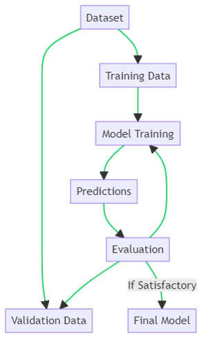
Supervised Learning Workflow
Data Splitting The dataset is divided into two subsets: Training Data, used to fit the model, and Validation Data, used to evaluate its predictive performance.
Model Training The Training Data is employed to train the model. This phase is analogous to a student studying lessons to acquire knowledge on a subject.
Predictions Once trained, the model applies the learned relationships to generate predictions on new inputs.
Evaluation Predictions are evaluated against the Validation Data to assess performance. This step functions like an examination, testing how well the model performs on data it has not encountered during training.
Refinement or Finalization
- If evaluation metrics indicate satisfactory performance, the model is finalized.
- If performance is inadequate, the model undergoes retraining. This iterative process continues until the desired predictive accuracy is achieved, similar to a student revising lessons to improve test scores.
Theoretical Framework
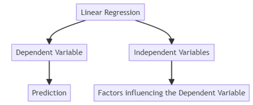
Simple Linear Regression (SLR)
Simple Linear Regression is a statistical method used to model the relationship between a single independent variable and a dependent variable. Its primary goal is to predict the dependent variable by fitting a straight line that minimizes the difference between predicted and observed values.
Simple Linear Regression
The mathematical form is:
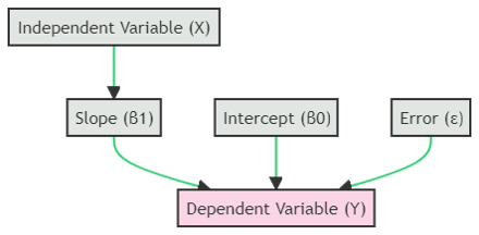
Linear Regression Equation
Y = β₀ + β₁X + ε
Where:
- Y (Dependent Variable): The outcome we want to predict, such as grades received.
- X (Independent Variable): The predictor, for example, hours studied.
- β₀ (Intercept): The expected value of Y when X is zero.
- β₁ (Slope): How much Y changes for each unit increase in X.
- ε (Error Term): The portion of Y not explained by X.
Example: In our case study, we predict students’ grades based on hours spent studying. The analysis reveals a positive correlation, meaning that, generally, as study hours increase, grades improve. The slope of the line quantifies this relationship, showing the expected increase in grades per additional hour of study.
Multiple Linear Regression (MLR)
Multiple Linear Regression generalizes SLR by allowing multiple independent variables to predict a single dependent variable. This approach captures more complex relationships and improves predictive accuracy by accounting for additional factors that influence the outcome.
The mathematical form is:
Multiple Linear Regression
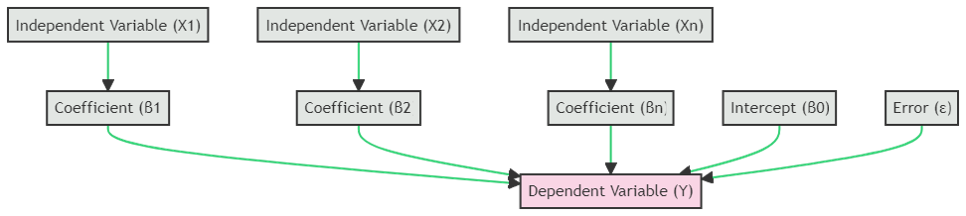
Y = β₀ + β₁x₁ + β₂x₂ + … + βₙxₙ + ε
Where:
- Y (Dependent Variable): The outcome we are predicting (grades).
- x₁, x₂, …, xₙ (Independent Variables): Multiple predictors, such as hours studied and hours of sleep.
- β₀ (Intercept): Value of Y when all predictors are zero.
- β₁, …, βₙ (Coefficients): Change in Y for a one-unit change in each predictor while keeping other variables constant.
- ε (Error Term): Variation in Y not explained by the predictors.
Example: Extending our study, suppose we include both hours studied and hours of sleep as predictors for grades. MLR models how both factors jointly influence performance. The resulting regression plane in three-dimensional space illustrates how changes in these two variables affect predicted grades. By considering multiple factors, MLR provides a more accurate and realistic prediction than SLR, especially when outcomes depend on more than one variable.
Methodology and Implementation
Experimental Setup (Python Implementation)
To demonstrate Simple Linear Regression, a Python model was implemented using scikit-learn to predict Grades Received based on Hours Studied.
Installation:
pip install scikit-learn matplotlib
Code Implementation:
import numpy as np
from sklearn.linear_model import LinearRegression
import matplotlib.pyplot as plt

# Dataset
hours_studied = np.array([1.0, 3.0, 2.3, 6.0, 1.5, 7.0, 5.0, 3.3, 4.0, 2.0, 3.0, 0.0, 5.5, 4.3]).reshape(-1, 1)
grades_received = np.array([35, 55, 42, 94, 36, 96, 90, 70, 80, 39, 50, 34, 95, 83])

# Create and fit model
model = LinearRegression()
model.fit(hours_studied, grades_received)

# Predictions
grades_predicted = model.predict(hours_studied)

# Visualization
plt.scatter(hours_studied, grades_received, color='black')
plt.plot(hours_studied, grades_predicted, color='blue', linewidth=3)
plt.xlabel('Hours Studied')
plt.ylabel('Grades Received')
plt.title('Linear Regression: Best Fit Line')
plt.show()

# Coefficients
print('Slope:', model.coef_[0])
print('Intercept:', model.intercept_)
Results and Visualization
The Simple Linear Regression implementation produces a “Best Fit Line” that demonstrates a positive correlation between study time and grades. The fitted line has a slope of 11.84 and an intercept of 23.68, indicating that each additional hour studied increases the predicted grade by approximately 11.84 points.
Output:
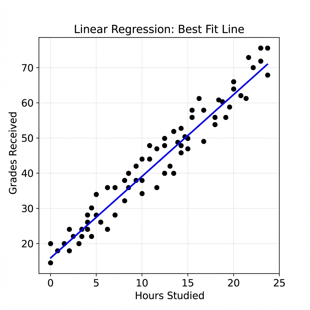
Linear Regression Plot
Slope: 11.84
Intercept: 23.68
In the context of Multiple Linear Regression, visualization extends to three dimensions. The regression plane, representing the relationship among two independent variables and a dependent variable, is demonstrated in the project’s supplementary video. The algorithm iteratively updates the weights (w₁, w₂) and bias (b) to minimize the Mean Squared Error (MSE). The initial MSE of 8313.18 converges substantially by iteration 49, confirming effective parameter optimization.
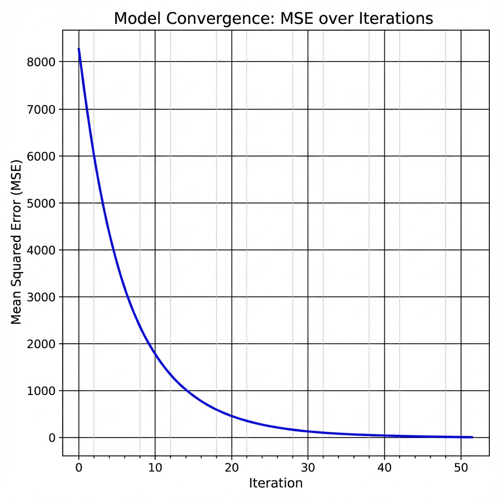
MSE Convergence Plot: Demonstrates iterative reduction in error during model training.
The animation below illustrates the convergence of the Multiple Linear Regression plane in three dimensions. It demonstrates how the model iteratively adjusts the weights and bias to minimize prediction error. The accompanying plot displays the progressive reduction of the Mean Squared Error over successive iterations.
3D visualization of Multiple Linear Regression convergence. The regression plane adjusts iteratively to fit the data points defined by two independent variables. The side plot displays the corresponding decrease in Mean Squared Error over successive iterations, illustrating the model’s optimization process.
ML Libraries
The successful implementation of the project utilized the following libraries:
Table 1: Library/Tool Used
| Tool/Library | Description |
|---|---|
| Scikit-Learn | Machine learning library for regression algorithms. |
| Numpy | Fundamental package for numerical computations. |
| Matplotlib | Plotting library for visualizing the regression line. |
Model Evaluation and Assumptions
Evaluation Metrics
The performance of a Multiple Linear Regression model is assessed using several statistical measures that quantify model fit and the relevance of individual predictors.
R-squared (R²) represents the proportion of variance in the dependent variable that is explained by the set of predictors. Values lie between 0 and 1. Higher values indicate that the model accounts for a greater share of the observed variability.
P-values used to evaluate the statistical significance of each coefficient. A p-value below 0.05 is commonly interpreted as evidence that the associated predictor contributes meaningfully to the model and should be retained.
Key Assumptions
The reliability of Multiple Linear Regression depends on satisfying several core assumptions. Violations can compromise coefficient estimates and reduce the interpretability of the model.
Table 2: Key Assumptions of Multiple Linear Regression
| Assumption | Description |
|---|---|
| Linearity | The relationship between each predictor and the response variable is assumed to be linear. |
| No Multicollinearity | Predictors should not exhibit high intercorrelation, since strong multicollinearity inflates variance and destabilizes coefficient estimates. |
| Homoscedasticity | Residuals should display constant variance across the range of fitted values. Unequal variance indicates heteroscedasticity and can affect inference. |
| Independence | Observations should be independent of one another. Dependence among data points can bias standard errors and test statistics. |
| Normality of Residuals | Model residuals are assumed to follow a normal distribution. This assumption supports valid hypothesis testing and confidence interval construction. |
Applications of Multiple Linear Regression
Multiple Linear Regression is widely used across many fields because it evaluates the distinct effect of several predictors on a continuous outcome. Its capacity to control for overlapping influences makes it a central method in quantitative analysis.
Finance
Multiple Linear Regression is used to model asset price behavior, estimate determinants of market returns, evaluate credit risk, and forecast macroeconomic variables. By incorporating multiple economic and firm-specific predictors, analysts can determine how each factor contributes to financial performance.
Healthcare
Clinical researchers apply Multiple Linear Regression to quantify relationships among risk factors and patient outcomes. It is frequently used to model disease progression, estimate the probability of hospitalization or readmission, and assess treatment effectiveness while adjusting for demographic and physiological variables.
Marketing and Consumer Analytics
In marketing, Multiple Linear Regression supports demand analysis, sales forecasting, and consumer behavior studies. Predictors such as pricing, promotional activity, demographic segments, and seasonal trends are evaluated to identify which variables exert the strongest influence on purchasing behavior or revenue patterns.
Social Sciences and Policy Research
Researchers use Multiple Linear Regression to study outcomes shaped by multiple societal influences, including educational performance, labor market participation, and housing dynamics. The model allows for more accurate interpretation of relationships within complex social systems.
Engineering and Environmental Sciences
Multiple Linear Regression is applied to predict system performance, estimate energy consumption, evaluate material properties, and analyze environmental indicators such as pollution levels or climate variability. These applications require simultaneous assessment of several interacting predictors.
Conclusion
Simple Linear Regression isolates the influence of a single predictor on a response variable, offering a narrow but interpretable view of their association. Multiple Linear Regression extends this framework by estimating the independent contribution of several predictors while controlling for mutual dependencies. This broader specification yields more informative parameter estimates, yet it also demands stricter diagnostic evaluation, particularly regarding multicollinearity, model specification error, and variance inflation. A clear understanding of these distinctions is essential for selecting an analytically sound regression approach and for drawing valid inferences from empirical data.
Presentation
Additional Resources
Project Source & Presentation Materials
Access the complete source code, presentation slides, and related machine learning materials via the repositories below:
Citation
Please cite this work as:
Thakur, Amey. "Multiple Linear Regression". AmeyArc (Sep 2023). https://amey-thakur.github.io/posts/2023-09-29-multiple-linear-regression/.Or use the BibTex citation:
@article{thakur2023mlr,
  title   = "Multiple Linear Regression",
  author  = "Thakur, Amey",
  journal = "amey-thakur.github.io",
  year    = "2023",
  month   = "Sep",
  url     = "https://amey-thakur.github.io/posts/2023-09-29-multiple-linear-regression/"
}