Special thanks to Mega Satish for her meaningful contributions, support, and wisdom that helped shape this work.
The core aim of this project is to take raw data, analyse it, and perform exploratory data analysis to clearly understand the underlying patterns. Using these insights, we build and train a Neural Network model to achieve accurate results. Finally, the complete system is deployed as a web application.
Abstract
Our project focuses on identifying a single SPY (S&P 500 ETF) investment strategy that maximises overall wealth. We compare our model’s performance with well-known approaches like the traditional buy-and-hold and the Moving Average Convergence Divergence (MACD) strategy. This work brings together Machine Learning, Data Science, and Web Development, with the final application deployed on the Heroku Cloud Platform.
The objective is to evaluate stock price behaviour based on essential market factors. We aim to forecast future price movements for specific stocks using historical price data and company-related financial news. Since reinforcement learning revolves around choosing optimal actions to maximise rewards, we use it here to predict stock closing prices based on past trends.
Using trained reinforcement learning models, we develop a multi-company predictor capable of estimating daily closing prices. By providing inputs such as open, high, and low prices, trading volume, and recent events related to each firm, the system determines the expected closing value for any given day.
Overall, this project is designed to build practical experience in Data Analytics, Machine Learning, and real-world model deployment.
Introduction
The stock market’s unpredictability has always fascinated us. With hundreds of stocks available and countless opportunities each day, the first challenge for a day trader is deciding what to trade. The next challenge is to identify strategies that can produce meaningful profit from these opportunities, whether in individual stocks, groups of stocks, or exchange-traded funds (ETFs).
Intraday traders use various techniques to capture short-term price movements. The best assets usually have high liquidity, noticeable volatility, and strong market participation. The main goal is to separate the actual market trend from surrounding noise and then take advantage of that trend at the correct moment.
Traditionally, traders relied on technical analysis, market sentiment, and current events to make trading decisions. With the growth of Data Science and Machine Learning, many of these time-consuming tasks can now be automated. Automated trading systems provide better timing, clearer insights, and more consistent predictions. They are especially useful for hedge funds and mutual funds, where even small improvements in accuracy can significantly improve returns. However, every profitable strategy comes with risk, and creating a reliable automated trading method is not simple.
Everyone who enters the stock market aims to maximise returns while keeping risk at a manageable level. To achieve this balance, reinforcement learning offers an effective approach. By learning from historical data, reinforcement learning agents can create trading strategies that adapt and improve over time.
This project was developed because we were interested in exploring these ideas and wanted practical experience with a Machine Learning project. It represents our attempt to understand how automated decision-making can be used to navigate the constantly changing environment of the stock market.
Reinforcement Learning
Reinforcement learning is a machine learning approach in which models learn to make a sequence of decisions. In an uncertain and often complex environment, the agent must figure out how to reach a specific goal. In reinforcement learning, artificial intelligence is placed in a game-like setting where it must experiment through trial and error to discover the best actions. The agent receives rewards or penalties based on its behaviour, which encourages it to perform actions that lead to the desired result. The aim is to maximise the total reward.
Although the designer defines the reward policy, which is essentially the set of rules for the task, the model is not given instructions or hints on how to solve it. The agent begins with random attempts and gradually learns more effective strategies, eventually developing advanced or even superhuman capabilities. It must discover the correct behaviour on its own in order to maximise its reward.
In reinforcement learning, developers use a framework that rewards useful actions and penalises harmful or unproductive ones. The agent receives positive values for desirable behaviour and negative values for undesirable behaviour. To find the optimal solution, the agent is encouraged to focus on long-term gains rather than short-term outcomes.
These long-term goals prevent the agent from getting stuck chasing smaller rewards. Over time, the agent learns to ignore negative patterns and continue reinforcing positive ones. This style of learning has been widely used in artificial intelligence to guide unsupervised behaviours through a system of rewards and penalties.
A simple example is teaching a dog. You allow the dog to behave freely, and when it does something good you say “Good dog.” When it misbehaves, you say “Bad dog.” Over time, the dog learns to repeat the good behaviours and avoid the bad ones.
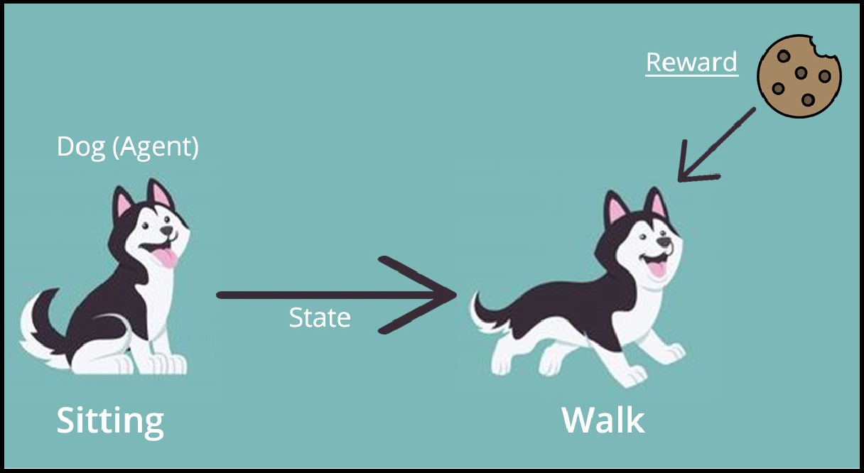
Example of teaching a dog
Trading is a continuous activity without a clear endpoint. Since we do not have complete information about market participants, trading can be viewed as a stochastic Markov Decision Process. We use model-free reinforcement learning, specifically Q-learning, because the reward function and transition probabilities are unknown.
Markov Decision Process (MDP)
A Markov Decision Process is a mathematical framework used to model decision-making problems where outcomes are partly random and partly influenced by the decision-maker. It is similar to a Markov chain because it predicts future outcomes based only on the current state. However, unlike a simple Markov chain, an MDP also considers the effect of actions and the rewards associated with those actions.
At each step, the decision-maker selects an action available in the current state. This action moves the system to the next state and results in a reward. Over time, the goal is to choose actions that maximise the total reward.
Markov Decision Process (MDP)
Machine learning algorithms often rely on MDPs when facing optimisation problems. In reinforcement learning, the agent interacts with an environment and aims to optimise its behaviour to achieve the highest possible long-term reward. While supervised learning requires correct input and output pairs, reinforcement learning uses the MDP framework to balance exploration and exploitation. This is useful when the probabilities of outcomes and the rewards associated with them are not fully known.
Terminologies
Agent The agent is the learner or decision-maker. It is the system we are training to make correct choices. For example, a robot being trained to move through a house without hitting obstacles.
Environment The environment is the world in which the agent operates. In the example above, the house is the robot’s environment. The agent cannot control the environment but can choose how to act within it. For instance, the robot cannot move a table, but it can walk around it.
State The state represents the current situation of the agent. It may include the robot’s exact location, its posture, or the orientation of its legs, depending on how the problem is defined.
Action Actions are the choices the agent can make at each time step. For example, moving its right leg, lifting an arm, turning left or right, or picking up an object. The set of possible actions is known in advance.
Policy A policy defines the agent’s strategy for choosing actions. In practice, it is a probability distribution over all possible actions. Actions that lead to higher rewards have a higher probability of being selected. Low-probability actions can still be chosen, but they are less likely.
Note: Even if an action has a low probability, it can still be selected. It simply has a lower chance of being chosen compared to actions with higher probabilities.
Q-Learning
The Q in Q-learning stands for quality. In this context, quality represents how effective a particular action is in obtaining a future reward. Q-learning is an off-policy reinforcement learning algorithm that aims to determine the best possible action to take in a given state. It is considered off-policy because it can learn from actions that do not follow the current policy, including random exploratory actions. As a result, Q-learning does not require a predefined policy. Its main objective is to learn a policy that maximises the total accumulated reward.
An agent interacts with the environment in two primary ways: exploitation and exploration. During exploitation, the agent evaluates all available actions and chooses the one that offers the highest expected reward based on its current knowledge. During exploration, the agent chooses a random action to discover new possibilities, without focusing on immediate reward. Over time, the agent builds a Q-table that stores the value of taking each action in each state, allowing it to make better decisions as learning progresses.
Points to Consider
Gamification of trading Historical and current prices, technical data, buy or sell or do nothing actions, and tracking profit and loss.
Train the system Treat each entry and exit as an individual game. Run through the price series both sequentially and randomly.
Reward function design Reward based on profit or loss at exit, otherwise zero, or cumulative profit and loss from the start of the trade to each time step.
Features to use Open, high, low, close, and volume (OHLCV), technical indicators, time of day, day of week, time of year, and different time granularities.
Test the system Use sine waves, trend curves, random walks, and add noise to clean test curves.
Types of deep learning algorithms Different architectures may be applied depending on the complexity of the environment and data.
Exploratory Data Analysis
In every Data Analysis or Data Science project, exploratory data analysis, or EDA, is a critical stage. EDA is the investigation of a dataset to find patterns and anomalies as well as to generate hypotheses based on our knowledge of the information.
During the course of a data science or machine learning project, EDA consumes around half of the time spent on data analysis, feature selection, feature engineering, and other processes. Because it is the most essential element or backbone of a data science project, where one has to perform several tasks like data cleaning, dealing with missing values, handling outliers, treating unbalanced datasets, handling categorical features, and many others. To automate our tasks in exploratory data analysis, we may utilise python packages like dtale, pandas profiling, sweetviz, and autoviz.
Create an Environment
In the reinforcement learning problem, the environment is a critical component. It’s critical to have a solid grasp of the underlying world with which the RL agent will interact. This aids us in developing the best design and learning strategy for the agent.
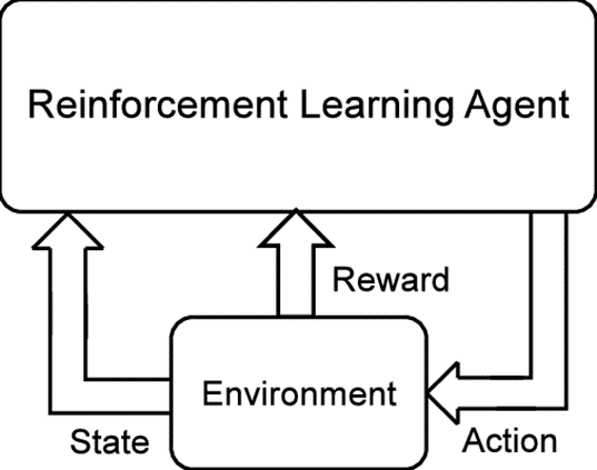
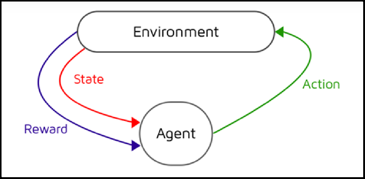
Reinforcement Learning Agent Environment Interaction
The reinforcement learning task is intended to be a simple framing of the challenge of learning from interaction in order to accomplish a goal. The agent is the learner and decision-maker. The environment is the object it interacts with, and it consists of everything outside the agent. The agent chooses actions, and the environment reacts to those actions, presenting the agent with new scenarios. The environment also produces rewards, which are unique numerical values that the agent attempts to maximise over time.
Stock Price Prediction with Deep Q-Learning (DQN)
This notebook implements a Reinforcement Learning (RL) agent to trade stocks. The agent uses a Deep Q-Network (DQN) to learn a trading strategy (Buy, Sell, or Hold) based on historical price differences.
Key Changes & Fixes from Original:
- Framework: Switched from
chainer(outdated) to PyTorch. - Data Splitting: Implemented a Time-Series Split (Train on past, Test on future) instead of random shuffling, which prevents data leakage.
- Interactive Logic: Removed blocking
input()calls to allow automated execution. - Visualization: Replaced
plotlywith Matplotlib for static rendering and reliability.
1. Imports and Setup
We import the necessary libraries. We use pandas for data manipulation, matplotlib for plotting, and torch for building the neural network.
Input:
import numpy as np
import pandas as pd
import matplotlib.pyplot as plt
import torch
import torch.nn as nn
import torch.optim as optim
import torch.nn.functional as F_torch
import copy
import time
import random
import json

# Set random seeds for reproducibility
torch.manual_seed(42)
np.random.seed(42)
random.seed(42)

print("Libraries imported successfully.")
Output:
Libraries imported successfully.
2. Data Loading and Preprocessing
We load the dataset and filter for a specific stock (e.g., ‘AAL’).
- Time-Series Split: We strictly split the data by date (
2016-01-01). The model trains on data before this date and is tested on data after it. This simulates real-world trading where you cannot see the future.
Input:
# Load dataset
data_path = 'all_stocks_5yr.csv'
data = pd.read_csv(data_path)

# Select a specific stock (e.g., American Airlines)
stock_name = 'AAL'
df = data[data['Name'] == stock_name].copy()

# Convert date column and sort
df['date'] = pd.to_datetime(df['date'])
df = df.set_index('date').sort_index()

# Split into Train and Test sets
date_split = '2016-01-01'
train = df[df.index < date_split]
test = df[df.index >= date_split]

print(f"Training Data: {len(train)} days")
print(f"Testing Data: {len(test)} days")
Output:
Training Data: 730 days
Testing Data: 529 days
3. Defining the Trading Environment
We create a custom environment class Environment1.
- State: The agent sees a history of price differences (returns) and its current unrealized profit/loss.
- Actions: 0 = Hold, 1 = Buy, 2 = Sell.
- Rewards: The agent receives a positive reward for selling at a profit and a negative reward for selling at a loss.
Input:
class Environment1:
    def __init__(self, df, history_t=90):
        self.data = df
        self.history_t = history_t
        self.reset()

    def reset(self):
        self.t = 0
        self.done = False
        self.profits = 0
        self.positions = []
        self.position_value = 0
        self.history = [0 for _ in range(self.history_t)]
        return [self.position_value] + self.history # Observation state

    def step(self, act):
        reward = 0

        # Actions: 0 = Stay, 1 = Buy, 2 = Sell
        if act == 1: # Buy
            self.positions.append(self.data.iloc[self.t]['close'])
        elif act == 2: # Sell
            if len(self.positions) == 0:
                reward = -1 # Penalty for invalid sell
            else:
                profits = 0
                for p in self.positions:
                    profits += (self.data.iloc[self.t]['close'] - p)
                reward += profits
                self.profits += profits
                self.positions = [] # Close all positions

        # Advance time
        self.t += 1

        # Calculate current position value (unrealized profit)
        self.position_value = 0
        for p in self.positions:
            self.position_value += (self.data.iloc[self.t]['close'] - p)

        # Update history (sliding window of price differences)
        self.history.pop(0)
        self.history.append(self.data.iloc[self.t]['close'] - self.data.iloc[(self.t-1)]['close'])

        # Clip Reward to stabilize training
        if reward > 0: reward = 1
        elif reward < 0: reward = -1

        # Check if end of dataset
        if self.t == len(self.data)-1:
            self.done = True

        return [self.position_value] + self.history, reward, self.done
4. Deep Q-Network (DQN) Model
We define a simple Feed-Forward Neural Network using PyTorch. It takes the environment state as input and outputs Q-values for the 3 possible actions.
Input:
class Q_Network(nn.Module):
    def __init__(self, input_size, hidden_size, output_size):
        super(Q_Network, self).__init__()
        self.fc1 = nn.Linear(input_size, hidden_size)
        self.fc2 = nn.Linear(hidden_size, hidden_size)
        self.fc3 = nn.Linear(hidden_size, output_size)

    def forward(self, x):
        h = F_torch.relu(self.fc1(x))
        h = F_torch.relu(self.fc2(h))
        y = self.fc3(h)
        return y
5. Training the Agent
This function trains the DQN agent using:
- Replay Memory: Stores past experiences to break correlation between samples.
- Target Network: A separate network to calculate target Q-values, improving stability.
- Epsilon-Greedy Strategy: Explores random actions initially and gradually shifts to exploiting the learned policy.
Input:
def train_dqn(env):
    # Hyperparameters
    input_size = env.history_t + 1
    hidden_size = 100
    output_size = 3
    epoch_num = 20        # Increase for better results
    memory_size = 200
    batch_size = 20
    gamma = 0.97
    epsilon = 1.0
    epsilon_min = 0.1
    epsilon_decrease = 1e-3

    # Initialize Networks
    Q = Q_Network(input_size, hidden_size, output_size)
    Q_ast = copy.deepcopy(Q) # Target Network
    optimizer = optim.Adam(Q.parameters(), lr=0.001)
    criterion = nn.MSELoss()

    memory = []
    total_losses = []
    total_rewards = []
    total_step = 0

    print("Starting training...")
    start_time = time.time()

    for epoch in range(epoch_num):
        pobs = env.reset()
        done = False
        epoch_reward = 0
        epoch_loss = 0

        while not done:
            # 1. Action Selection (Epsilon Greedy)
            pact = np.random.randint(3)
            if np.random.rand() > epsilon:
                pobs_tensor = torch.tensor(pobs, dtype=torch.float32).unsqueeze(0)
                with torch.no_grad():
                    pact = torch.argmax(Q(pobs_tensor)).item()

            # 2. Step in Environment
            obs, reward, done = env.step(pact)

            # 3. Store in Memory
            memory.append((pobs, pact, reward, obs, done))
            if len(memory) > memory_size:
                memory.pop(0)

            # 4. Train Experience Replay
            if len(memory) == memory_size and total_step % 10 == 0:
                batch = random.sample(memory, batch_size)

                b_pobs = torch.tensor([x[0] for x in batch], dtype=torch.float32)
                b_pact = torch.tensor([x[1] for x in batch], dtype=torch.int64)
                b_reward = torch.tensor([x[2] for x in batch], dtype=torch.float32)
                b_obs = torch.tensor([x[3] for x in batch], dtype=torch.float32)
                b_done = torch.tensor([x[4] for x in batch], dtype=torch.float32)

                # Current Q values
                q_pred = Q(b_pobs).gather(1, b_pact.unsqueeze(1)).squeeze(1)

                # Target Q values
                with torch.no_grad():
                    maxq_next = torch.max(Q_ast(b_obs), dim=1)[0]
                    target = b_reward + gamma * maxq_next * (1 - b_done)

                loss = criterion(q_pred, target)
                epoch_loss += loss.item()

                optimizer.zero_grad()
                loss.backward()
                optimizer.step()

                # Update Target Network
                if total_step % 20 == 0:
                    Q_ast = copy.deepcopy(Q)

            # Update Epsilon
            if epsilon > epsilon_min and total_step > 200:
                epsilon -= epsilon_decrease

            pobs = obs
            epoch_reward += reward
            total_step += 1

        total_rewards.append(epoch_reward)
        total_losses.append(epoch_loss)

        if (epoch+1) % 5 == 0:
            print(f"Epoch {epoch+1}/{epoch_num} | Reward: {epoch_reward} | Loss: {epoch_loss:.2f} | Epsilon: {epsilon:.2f}")

    print(f"Training finished in {time.time() - start_time:.2f} seconds.")
    return Q, total_losses, total_rewards

# Run Training
train_env = Environment1(train)
Q_model, losses, rewards = train_dqn(train_env)
Output:
Starting training...
Epoch 5/20 | Reward: 8 | Loss: 2837.32 | Epsilon: 0.10
Epoch 10/20 | Reward: -24 | Loss: 174.92 | Epsilon: 0.10
Epoch 15/20 | Reward: -44 | Loss: 619.27 | Epsilon: 0.10
Epoch 20/20 | Reward: -9 | Loss: 21.38 | Epsilon: 0.10
Training finished in 14.99 seconds.
6. Evaluation and Visualization
We visualize the agent’s performance on both Training and Testing data.
- Blue Line: Training Data (Past)
- Orange Line: Testing Data (Future)
- Green/Red Markers: Buy and Sell actions taken by the trained agent.
Input:
def plot_results(train_env, test_env, Q):
    # Helper to get actions from the model
    def run_inference(env):
        pobs = env.reset()
        acts = []
        for _ in range(len(env.data)-1):
            pobs_tensor = torch.tensor(pobs, dtype=torch.float32).unsqueeze(0)
            with torch.no_grad():
                pact = torch.argmax(Q(pobs_tensor)).item()
            acts.append(pact)
            pobs, _, _ = env.step(pact)[0:3]
        return acts

    train_acts = run_inference(train_env)
    test_acts = run_inference(test_env)

    plt.figure(figsize=(15, 6))

    # Plot Train Data
    plt.plot(train_env.data.index, train_env.data['close'], label='Train Data', color='blue', alpha=0.5)

    # Plot Test Data
    plt.plot(test_env.data.index, test_env.data['close'], label='Test Data', color='orange', alpha=0.5)

    # Mark Buy/Sell Points
    def plot_markers(dates, close_prices, acts, label_prefix):
        buy_idx = [i for i, x in enumerate(acts) if x == 1]
        sell_idx = [i for i, x in enumerate(acts) if x == 2]

        if buy_idx:
            plt.scatter(dates[buy_idx], close_prices.iloc[buy_idx],
                       marker='^', color='green', s=30, label=f'{label_prefix} Buy')
        if sell_idx:
            plt.scatter(dates[sell_idx], close_prices.iloc[sell_idx],
                       marker='v', color='red', s=30, label=f'{label_prefix} Sell')

    plot_markers(train_env.data.index, train_env.data['close'], train_acts, 'Train')
    plot_markers(test_env.data.index, test_env.data['close'], test_acts, 'Test')

    plt.axvline(x=pd.to_datetime(date_split), color='black', linestyle='--', label='Train/Test Split')
    plt.title(f'DQN Trading Agent on {stock_name}')
    plt.legend()
    plt.show()

    print(f"Final Train Profit: {train_env.profits:.2f}")
    print(f"Final Test Profit: {test_env.profits:.2f}")

# Visualize
test_env = Environment1(test)
plot_results(train_env, test_env, Q_model)
Output:
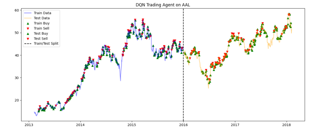
DQN Trading Agent on AAL
Final Train Profit: 251.91
Final Test Profit: 127.90
Results
WEB APPLICATION - https://stock-trading-with-rl.herokuapp.com
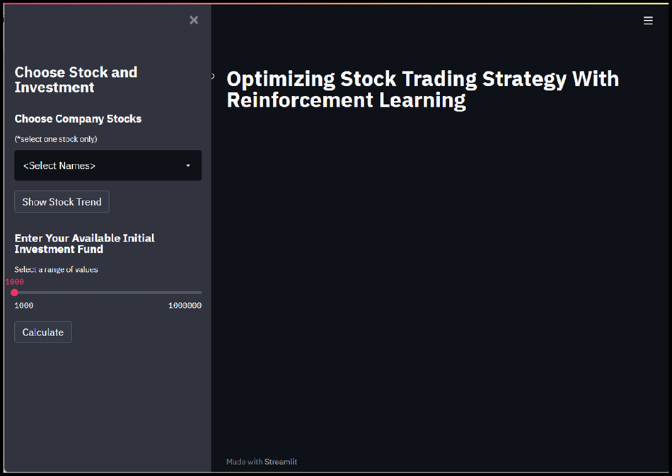
Web Application Interface
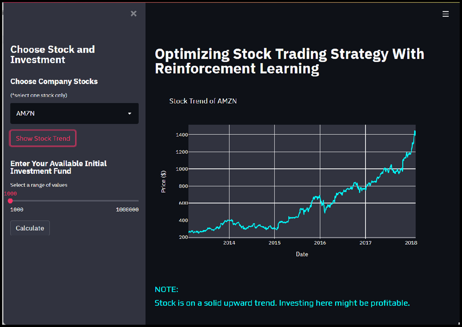
Stock Trend Visualization
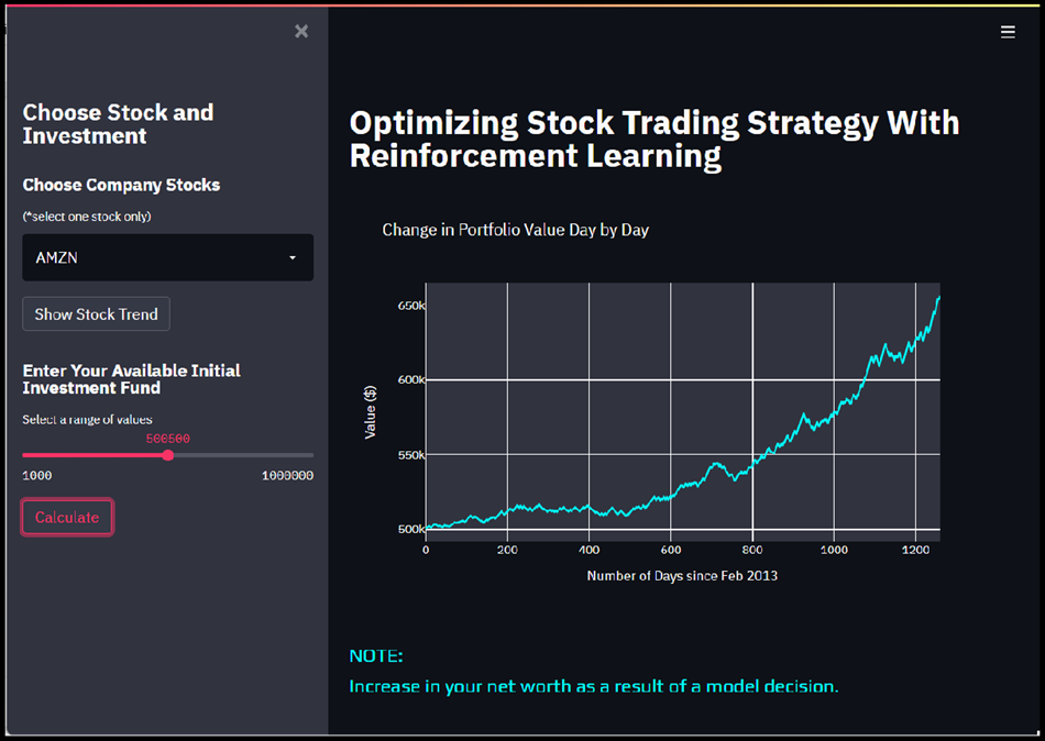
Portfolio Value Visualization
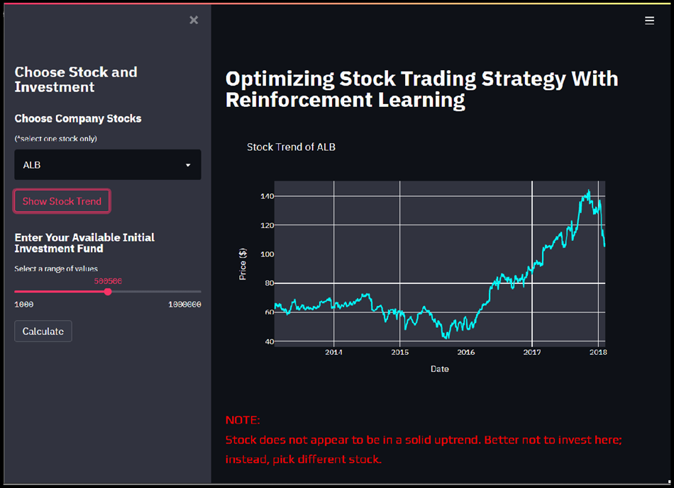
Stock Trend Visualization (Downtrend)
YouTube Demonstration
Presentation
Additional Resources
Project Source, Notebooks, Research & Demonstrations
Explore the complete source code, Kaggle notebooks, research publications, and video demonstrations for the Optimizing Stock Trading Strategy project via the resources below:
Citation
Please cite this work as:
Thakur, Amey. "Optimizing Stock Trading Strategy With Reinforcement Learning". AmeyArc (Sep 2021). https://amey-thakur.github.io/posts/2021-09-22-optimizing-stock-trading-strategy-with-reinforcement-learning/.Or use the BibTex citation:
@article{thakur2021stocktrading,
  title   = "Optimizing Stock Trading Strategy With Reinforcement Learning",
  author  = "Thakur, Amey",
  journal = "amey-thakur.github.io",
  year    = "2021",
  month   = "Sep",
  url     = "https://amey-thakur.github.io/posts/2021-09-22-optimizing-stock-trading-strategy-with-reinforcement-learning/"
}