Special thanks to Mega Satish for her meaningful contributions, support, and wisdom that helped shape this work.
We propose to implement a house price prediction model of Bangalore, India. It’s a Machine Learning model which integrates Data Science and Web Development. We have deployed the app on the Heroku Cloud Application Platform. Housing prices fluctuate on a daily basis and are sometimes exaggerated rather than based on worth. The major focus of this project is on predicting home prices using genuine factors. Here, we intend to base an evaluation on every basic criterion that is taken into account when establishing the pricing. The goal of this project is to learn Python and get experience in Data Analytics, Machine Learning, and AI.
Introduction
Context
This project was made because we were intrigued and we wanted to gain hands-on experience with the Machine Learning Project.
Motivation
We are highly interested in anything related to Machine Learning, the independent project provided us with the opportunity to study and reaffirm our passion for this subject. The capacity to generate guesses, forecasts, and offer machines the ability to learn on their own is both powerful and infinite in terms of application possibilities. Machine Learning may be applied in finance, medicine, and virtually any other field. That is why we opted to base our idea on Machine Learning.
Objective
As a first project, we intended to make it as instructional as possible by tackling each stage of the machine learning process and attempting to comprehend it well. We have picked Bangalore Real Estate Prediction as a method, which is known as a “toy issue,” identifying problems that are not of immediate scientific relevance but are helpful to demonstrate and practice. The objective was to forecast the price of a specific apartment based on market pricing while accounting for various “features” that would be established in the following sections.
Literature Survey
Real Estate Property is not only a person’s primary desire, but it also reflects a person’s wealth and prestige in today’s society. Real estate investment typically appears to be lucrative since property values do not drop in a choppy fashion. Changes in the value of the real estate will have an impact on many home investors, bankers, policymakers, and others. Real estate investing appears to be a tempting option for investors. As a result, anticipating the important estate price is an essential economic indicator. According to the 2011 census, the Asian country ranks second in the world in terms of the number of households, with a total of 24.67 crores. However, previous recessions have demonstrated that real estate costs cannot be seen. The expenses of significant estate property are linked to the state’s economic situation. Regardless, we don’t have accurate standardized approaches to live the significant estate property values.
First, we looked at different articles and discussions about machine learning for housing price prediction. The title of the article is house price prediction, and it is based on machine learning and neural networks. The publication’s description is minimal error and the highest accuracy. The aforementioned title of the paper is Hedonic models based on price data from Belfast infer that submarkets and residential valuation this model is used to identify over a larger spatial scale and implications for the evaluation process related to the selection of comparable evidence and the quality of variables that the values may require. Understanding current developments in house prices and homeownership are the subject of the study. In this article, they utilized a feedback mechanism or social pandemic that fosters a perception of property as an essential market investment.
Methodology
Data Collection
The statistics were gathered from Bangalore home prices. The information includes many variables such as area type, availability, location, BHK, society, total square feet, bathrooms, and balconies.
Linear Regression
Linear regression is a supervised learning technique. It is responsible for predicting the value of a dependent variable (Y) based on a given independent variable (X). It is the connection between the input (X) and the output (Y). It is one of the most well-known and well-understood machine learning algorithms. Simple linear regression, ordinary least squares, Gradient Descent, and Regularization are the linear regression models.
Decision Tree Regression
It is an object that trains a tree-structured model to predict data in the future in order to provide meaningful continuous output. The core principles of decision trees, Maximizing Information Gain, Classification trees, and Regression trees are the processes involved in decision tree regression. The essential notion of decision trees is that they are built via recursive partitioning. Each node can be divided into child nodes, beginning with the root node, which is known as the parent node. These nodes have the potential to become the parent nodes of their resulting offspring nodes. The nodes at the informative features are specified as the maximizing information gain, to establish an objective function that is to optimize the tree learning method.
Classification Trees
Classification trees are used to forecast the object into classes of a categorical dependent variable based on one or more predictor variables.
Regression Trees
It supports both continuous and categorical input variables. Regression trees are regarded as research with various machine algorithms for the regression issue, with the Decision Tree approach providing the lowest loss. The R-Squared value for the Decision Tree is 0.998, indicating that it is an excellent model. The Decision Tree was used to complete the web development.
Support Vector Regression
Supervised learning is linked with learning algorithms that examine data for classification and regression analysis.
Random Forest Regression
It is an essential learning approach for classification and regression to create a large number of decision trees. Preliminaries of decision trees are common approaches for a variety of machine learning problems. Tree learning is required for serving n off the self-produce for data mining since it is invariant despite scaling and several other changes. The trees are grown very deep in order to learn a high regular pattern. Random forest is a method of averaging several deep decision trees trained on various portions of the same training set. This comes at the price of a slight increase in bias and some interoperability.
Project
Problem Statement
Create a model to estimate the price of houses in Bengaluru and host it on Heroku.
Data
The data is the most important aspect of a machine learning assignment, to which special attention should be paid. Indeed, the data will heavily affect the findings depending on where we found them, how they are presented, if they are consistent, if there is an outlier, and so on. Many questions must be addressed at this stage to ensure that the learning algorithm is efficient and correct. To obtain, clean, and convert the data, many sub steps are required. We will go through these steps to understand how they’ve been used in my project and why they’re helpful for the machine learning section.
Dataset
Dataset: https://www.kaggle.com/ameythakur20/bangalore-house-prices
Model
Model: https://www.kaggle.com/ameythakur20/bangalore-house-price-prediction-model
Project Architecture
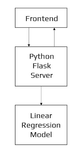
Architecture of the Application
Data Science
The first stage is standard data science work, in which we take a data set named ‘Bengaluru House pricing data’ from Kaggle. We will do significant data cleaning on it to guarantee that it provides reliable predictions throughout prediction. This Jupyter notebook, ‘Bangalore-House-Price-Prediction-Model.ipynb,’ is where we do all of our data science work. Because the Jupyter notebook is self-explanatory, we will only touch on the principles that we have implemented briefly. In terms of data cleansing, our dataset needs a significant amount of effort. In fact, 70% of the notebook is dedicated to data cleaning, in which we eliminate empty rows and remove superfluous columns that will not aid in prediction. The process of obtaining valuable and significant information from a dataset that will contribute the most to a successful prediction is the next stage. The final stage is to deal with outliers. Outliers are abnormalities that do massive damage to data and prediction. There is a lot to comprehend conceptually from the dataset in order to discover and eliminate these outliers. Finally, the original dataset of over 13000 rows and 9 columns is reduced to about 7000 rows and 5 columns.
Machine Learning
The resulting data is fed into a machine learning model. To find the optimal procedure and parameters for the model, we will mostly employ K-fold Cross-Validation and the GridSearchCV approach. It turns out that the linear regression model produces the best results for our data, with a score of more than 80%, which is not terrible. Now, we need to export our model as a pickle file (Bengaluru_House_Data.pickle), which transforms Python objects into a character stream. Also, in order to interact with the locations(columns) from the frontend, we must export them into a JSON (columns.json) file.
Frontend
The front end is built up of straightforward HTML. To receive an estimated pricing, the user may fill-up the form with the number of square feet, BHK, bathrooms, and location and click the ‘ESTIMATE PRICE’ button. We have used Flask Server and configured it in python. It takes the form data entered by the user and executes the function, which employs the prediction model to calculate the projected price in lakhs of rupees (1 lakh = 100000).
Experimental Setup
Steps to Create Model
Import Libraries
We import the necessary libraries for data manipulation, mathematical operations, and plotting.
Input:
import pandas as pd
import numpy as np
from matplotlib import pyplot as plt
import matplotlib
%matplotlib inline
matplotlib.rcParams["figure.figsize"] = (20,10)
Load Dataset
Load the CSV file into a Pandas DataFrame.
Input:
df1 = pd.read_csv("/kaggle/input/bangalore-house-prices/bengaluru_house_prices.csv")
print(df1.head())
Output:
    area_type   availability                  location       size  \
0  Super built-up  Area         19-Dec  Electronic City Phase II      2 BHK
1            Plot  Area  Ready To Move          Chikka Tirupathi  4 Bedroom
2        Built-up  Area  Ready To Move               Uttarahalli      3 BHK
3  Super built-up  Area  Ready To Move        Lingadheeranahalli      3 BHK
4  Super built-up  Area  Ready To Move                  Kothanur      2 BHK

   society total_sqft  bath  balcony   price
0  Coomee        1056   2.0      1.0   39.07
1  Theanmp       2600   5.0      3.0  120.00
2      NaN       1440   2.0      3.0   62.00
3  Soiewre       1521   3.0      1.0   95.00
4      NaN       1200   2.0      1.0   51.00
Exploratory Data Analysis
Understand the data structure, shape, and count of unique values.
Input:
print("Shape:", df1.shape)
print("Columns:", df1.columns)
print(df1.groupby('area_type')['area_type'].agg('count'))
Output:
Shape: (13320, 9)
Columns: Index(['area_type', 'availability', 'location', 'size', 'society',
       'total_sqft', 'bath', 'balcony', 'price'],
      dtype='object')
area_type
Built-up  Area          2418
Carpet  Area              87
Plot  Area              2025
Super built-up  Area    8790
Name: area_type, dtype: int64
Data Cleaning
Drop unnecessary columns and handle missing values. We also fix the format of the size and total_sqft columns.
Input:
# Drop unnecessary columns
df2 = df1.drop(['area_type','society','balcony','availability'], axis='columns')

# Drop missing values AND create a fresh copy to avoid SettingWithCopyWarning
df3 = df2.dropna().copy()

# Fix 'size' column (e.g., convert "2 BHK" to 2)
# Now this line will work without warnings because df3 is an independent copy
df3['bhk'] = df3['size'].apply(lambda x: int(x.split(' ')[0]))

# Fix 'total_sqft' column (convert ranges like "1133 - 1384" to average)
def convert_sqft_to_num(x):
    tokens = x.split('-')
    if len(tokens) == 2:
        return (float(tokens[0]) + float(tokens[1])) / 2
    try:
        return float(x)
    except:
        return None

df4 = df3.copy()
df4['total_sqft'] = df4['total_sqft'].apply(convert_sqft_to_num)
df4 = df4.dropna()
Feature Engineering
Create a new feature price_per_sqft which helps in outlier detection later.
Input:
df5 = df4.copy()
df5['price_per_sqft'] = df5['price'] * 100000 / df5['total_sqft']
print(df5.head())
Output:
    location       size  total_sqft  bath   price  bhk  \
0  Electronic City Phase II      2 BHK      1056.0   2.0   39.07    2
1          Chikka Tirupathi  4 Bedroom      2600.0   5.0  120.00    4
2               Uttarahalli      3 BHK      1440.0   2.0   62.00    3
3        Lingadheeranahalli      3 BHK      1521.0   3.0   95.00    3
4                  Kothanur      2 BHK      1200.0   2.0   51.00    2

   price_per_sqft
0     3699.810606
1     4615.384615
2     4305.555556
3     6245.890861
4     4250.000000
Dimensionality Reductions
Group locations with very few data points (less than 10) into a single category called “other” to reduce the number of columns when we do One Hot Encoding.
Input:
df5.location = df5.location.apply(lambda x: x.strip())
location_stats = df5.groupby('location')['location'].agg('count').sort_values(ascending=False)

location_stats_less_than_10 = location_stats[location_stats<=10]

df5.location = df5.location.apply(lambda x: 'other' if x in location_stats_less_than_10 else x)
print("Total unique locations:", len(df5.location.unique()))
Output:
Total unique locations: 241Outlier Removal using Business Logic
Remove properties where the square footage per bedroom is suspiciously low (less than 300 sqft per bedroom).
Input:
df6 = df5[~(df5.total_sqft/df5.bhk < 300)]
print("Shape after business logic removal:", df6.shape)
Output:
Shape after business logic removal: (12456, 7)Outlier Removal using Standard Deviation & Mean
We remove properties where the price per sqft is extremely high or low compared to other properties in the same location (using Mean and Standard Deviation). We also remove 2 BHK apartments that are more expensive than 3 BHK apartments in the same area.
Input:
# Filter by Price Per Sqft (Mean +/- 1 Std Dev)
def remove_pps_outliers(df):
    df_out = pd.DataFrame()
    for key, subdf in df.groupby('location'):
        m = np.mean(subdf.price_per_sqft)
        st = np.std(subdf.price_per_sqft)
        reduced_df = subdf[(subdf.price_per_sqft>(m-st)) & (subdf.price_per_sqft<=(m+st))]
        df_out = pd.concat([df_out,reduced_df],ignore_index=True)
    return df_out

df7 = remove_pps_outliers(df6)

# Filter by BHK Price (Remove 2 BHK > 3 BHK price)
def remove_bhk_outliers(df):
    exclude_indices = np.array([])
    for location, location_df in df.groupby('location'):
        bhk_stats = {}
        for bhk, bhk_df in location_df.groupby('bhk'):
            bhk_stats[bhk] = {
                'mean': np.mean(bhk_df.price_per_sqft),
                'std': np.std(bhk_df.price_per_sqft),
                'count': bhk_df.shape[0]
            }
        for bhk, bhk_df in location_df.groupby('bhk'):
            stats = bhk_stats.get(bhk-1)
            if stats and stats['count']>5:
                exclude_indices = np.append(exclude_indices, bhk_df[bhk_df.price_per_sqft<(stats['mean'])].index.values)
    return df.drop(exclude_indices,axis='index')

df8 = remove_bhk_outliers(df7)
print("Shape after all outlier removal:", df8.shape)
Output:
Shape after all outlier removal: (7317, 7)Data Visualization
Visualize the data to see the spread of 2 BHK vs 3 BHK prices and the distribution of Price Per Sqft.
Input:
def plot_scatter_chart(df,location):
    bhk2 = df[(df.location==location) & (df.bhk==2)]
    bhk3 = df[(df.location==location) & (df.bhk==3)]
    matplotlib.rcParams['figure.figsize'] = (15,10)
    plt.scatter(bhk2.total_sqft,bhk2.price,color='blue',label='2 BHK', s=50)
    plt.scatter(bhk3.total_sqft,bhk3.price,marker='+', color='green',label='3 BHK', s=50)
    plt.xlabel("Total Square Feet Area")
    plt.ylabel("Price (Lakh Indian Rupees)")
    plt.title(location)
    plt.legend()

# Scatter Plot
plot_scatter_chart(df8,"Rajaji Nagar")

# Histogram
import matplotlib
matplotlib.rcParams["figure.figsize"] = (20,10)
plt.hist(df8.price_per_sqft,rwidth=0.8)
plt.xlabel("Price Per Square Feet")
plt.ylabel("Count")
plt.show()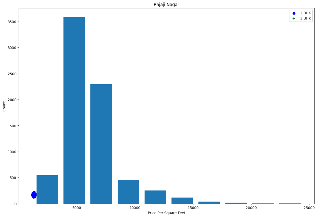
Data Visualization
Building a Model
Prepare the data (One Hot Encoding), split into training and testing sets, and train a Linear Regression model.
Input:
# Drop helper columns and filter outliers one last time
df9 = df8[df8.price_per_sqft<10000]
df10 = df9.drop(['price_per_sqft'],axis='columns')

# One Hot Encoding
dummies = pd.get_dummies(df10.location)
df11 = pd.concat([df10,dummies.drop('other',axis='columns')],axis='columns')

# FIX: Drop both 'location' AND 'size' columns
df12 = df11.drop(['location', 'size'], axis='columns')

# Define X and y
X = df12.drop('price',axis='columns')
y = df12.price

# Train Test Split
from sklearn.model_selection import train_test_split
X_train, X_test, y_train, y_test = train_test_split(X,y,test_size=0.2,random_state=10)

# Train Linear Regression
from sklearn.linear_model import LinearRegression
lr_clf = LinearRegression()
lr_clf.fit(X_train,y_train)
print("Model Score:", lr_clf.score(X_test,y_test))
Output:
Model Score: 0.8980700692588083Test the Model for few properties
Create a helper function to predict prices for arbitrary locations and features.
Input:
def predict_price(location, sqft, bath, bhk):
    # Find the index of the location column
    # If location is not found (e.g., it's 'other'), this block is skipped safely
    try:
        loc_index = np.where(X.columns == location)[0][0]
    except IndexError:
        loc_index = -1

    # Create an array of zeros with the same number of columns as X
    x = np.zeros(len(X.columns))
    x[0] = sqft
    x[1] = bath
    x[2] = bhk

    # Set the location column to 1 if it exists
    if loc_index >= 0:
        x[loc_index] = 1

    # FIX: Create a DataFrame with column names to match training data
    x_df = pd.DataFrame([x], columns=X.columns)

    return lr_clf.predict(x_df)[0]

# Test again
print("Prediction 1:", predict_price('1st Phase JP Nagar', 1000, 2, 2))
print("Prediction 2:", predict_price('1st Phase JP Nagar', 1000, 3, 3))
print("Prediction 3:", predict_price('Indira Nagar', 1000, 2, 2))
Output:
Prediction 1: 84.25840465992951
Prediction 2: 84.87720242072712
Prediction 3: 85.22387691807114
Export the tested model to a pickle file
Save the model and column information for use in deployment.
Input:
import pickle
with open('banglore_home_prices_model.pickle','wb') as f:
    pickle.dump(lr_clf,f)

import json
columns = {
    'data_columns' : [col.lower() for col in X.columns]
}
with open("columns.json","w") as f:
    f.write(json.dumps(columns))
print("Export complete.")
Output:
Export complete.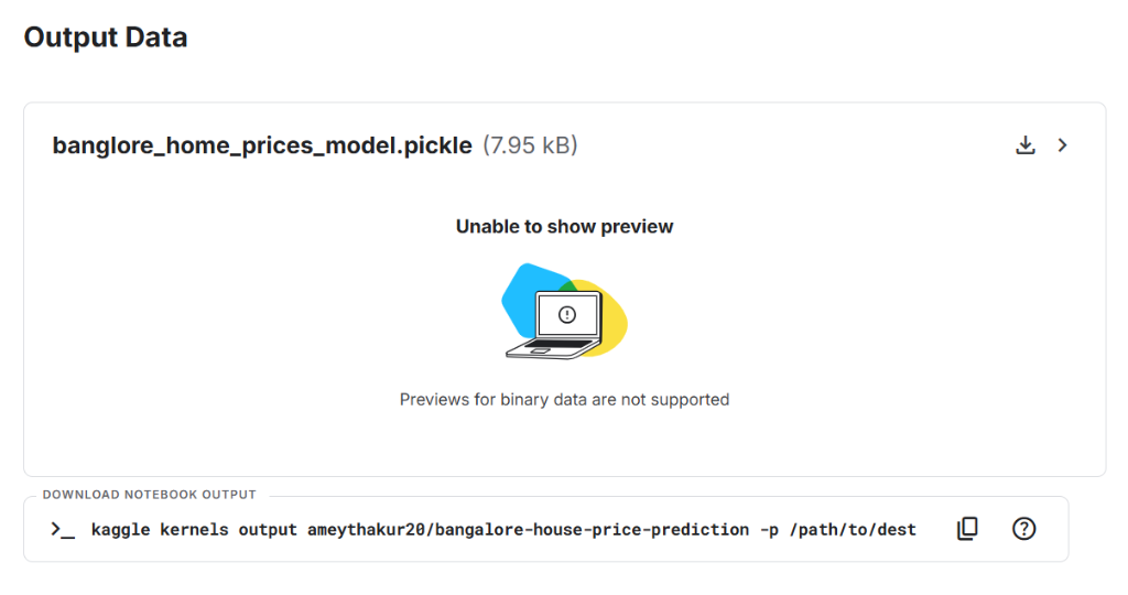
Output Data
Prerequisites
Before running these commands, ensure you have the following files in your project folder:
- app.py: Your Python Flask/Streamlit application file.
- requirements.txt: A list of libraries your app needs (e.g., scikit-learn, pandas, flask, gunicorn).
- Procfile: A file named exactly
Procfile(no extension) containing the command to start your app (e.g.,web: gunicorn app:app).
Steps to Deploy Model on Heroku
Login to Heroku
Connect your terminal to your Heroku account. It will open a browser window for you to log in.
heroku loginInitialize Git Repository
Initialize a new empty Git repository inside your project folder.
git initCreate Heroku App
Create a new application space on Heroku.
Note: The repository name
bangalorehousepricepredictionis already taken by me. Please add your name or a numeric suffix to make it unique (for example,bangalore-price-pred-amey).heroku create bangalorehousepricepredictionAdd Files to Git
Stage all your files (model, python scripts, requirements) for the commit.
git add .Commit Changes
Save your changes to the local git repository with a message.
git commit -am "initial commit"Push to Heroku
Upload your code to Heroku’s remote server. This triggers the building and deployment process.
git push heroku master(If you are using a newer version of Git where the default branch is
maininstead ofmaster, usegit push heroku main)
Tools used
Table 1: Tools Used
| Tool | Description |
|---|---|
| Anaconda | Python distribution for managing data science libraries and environments. |
| Jupyter Notebook | Interactive environment for experimentation, analysis, and model development. |
| Google Colab | Cloud-based notebooks for training and testing with scalable compute. |
| Flask | Lightweight web framework used to build the backend server. |
| Heroku | Platform-as-a-Service (PaaS) for application deployment. |
Technologies used
Table 2: Technologies Used
| Technology | Description |
|---|---|
| Python | Core language for model development and backend logic. |
| HTML | Markup for structuring the web interface. |
| CSS | Styling and layout of the frontend. |
| Bootstrap | Framework for responsive and consistent UI design. |
Results
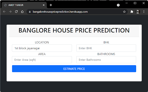
User Interface
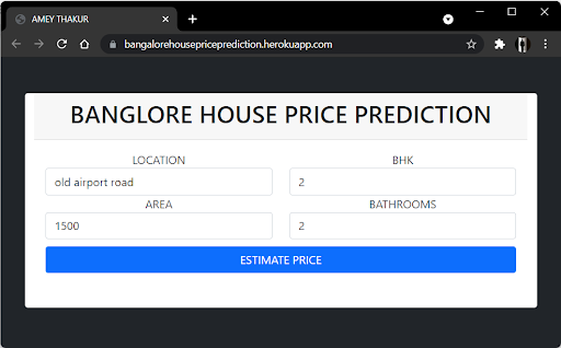
Estimate Price
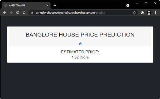
Predict
Heroku Web Application - https://bhpp.herokuapp.com, https://bangalorehousepriceprediction.herokuapp.com
YouTube Demonstration
Additional Resources
Project Source, Research & Demonstrations
Explore the complete source code, Kaggle notebooks, research publications, and video demonstrations for the Bangalore House Price Prediction project via the resources below:
Citation
Please cite this work as:
Thakur, Amey. "Bangalore House Price Prediction". AmeyArc (Sep 2021). https://amey-thakur.github.io/posts/2021-09-07-bangalore-house-price-prediction/.Or use the BibTex citation:
@article{thakur2021houseprice,
  title   = "Bangalore House Price Prediction",
  author  = "Thakur, Amey",
  journal = "amey-thakur.github.io",
  year    = "2021",
  month   = "Sep",
  url     = "https://amey-thakur.github.io/posts/2021-09-07-bangalore-house-price-prediction/"
}