Special thanks to Mega Satish for her meaningful contributions, support, and wisdom that helped shape this work.
Deep learning’s breakthrough in the field of artificial intelligence has resulted in the creation of a slew of deep learning models. One of these is the Generative Adversarial Network, which has only recently emerged. The goal of GAN is to use unsupervised learning to analyse the distribution of data and create more accurate results. The GAN allows the learning of deep representations in the absence of substantial labelled training information. Computer vision, language and video processing, and image synthesis are just a few of the applications that might benefit from these representations. The purpose of this research is to get the reader conversant with the GAN framework as well as to provide the background information on Generative Adversarial Networks, including the structure of both the generator and discriminator, as well as the various GAN variants along with their respective architectures. Applications of GANs are also discussed with examples.
Introduction
In the last decade, the rise of machine learning and later deep learning has taken an essential role in the field of computer science. With this breakthrough, our ability to solve complex problems continues to increase significantly. Deep learning has the potential of discovering comprehensive multilayer models [1] capable of describing probabilities for data used in artificial intelligence applications. Generative Adversarial Networks [2][3] are a type of generative modelling that employs deep learning techniques such as convolutional neural networks. GANs are a revolutionary innovation for both kinds of learning, supervised and unsupervised. GANs [4] are a creative approach to train a generative model by defining it as a supervised learning technique with two sub-models: the generator model, which we train to create new instances, and the discriminator model, which attempts to categorise examples as real or fake i.e. generated. The two models are trained until the discriminator model is tricked approximately half of the time, indicating that the generator model is producing convincing instances.
In machine learning, generative modelling is an unsupervised learning problem that entails automatically identifying and trying to learn patterns or similarities in the dataset so that the model may be used to create or produce new instances that might have been drawn from the original dataset. In Generative Adversarial Networks, the generator creates a new sample from input data and the discriminator tries to distinguish whether the generated sample is real or fake. Both networks are in competition with one another and are being trained at the same time. The generator doesn’t know how to generate the sample; it learns by interacting with the discriminator. The discriminator basically tries to distinguish between the sample generated by the generator model and the actual data as it has access to both real data and synthesized data. If the output of the generator is considered fake, an error signal is sent to the generator to improve the quality of the results. The discriminator is then modified in the following round to improve its ability to distinguish between real and false data, and the generator is changed depending on how successfully or poorly the produced samples deceived the discriminator.
With this paper, we are proposing an explanation of Generative Adversarial Networks background as well as generative modelling and discriminative modelling. We intend to describe the architecture of the Generative Adversarial Network including its working and the data used for this system. We aim to provide an elucidation of the variations of GANs along with their applications in the real world.
Supervised and Unsupervised Learning
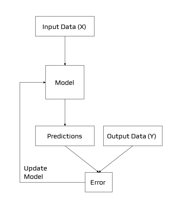
Predictive modelling, for example, is a common machine learning issue that includes utilising a model to generate a forecast. This necessitates a training dataset, which consists of numerous instances, referred to as samples, each having input variables (X) and output class labels (y). A model is trained by displaying patterns of inputs, having it predict outputs, and then correcting the model so that the outputs are more similar to the predicted outputs [5]. A supervised type of learning, or supervised learning [6], refers to the process of correcting the model. Classification and regression are examples of supervised learning tasks, whereas logistic regression and random forest are examples of supervised learning algorithms.
Example of Supervised Learning
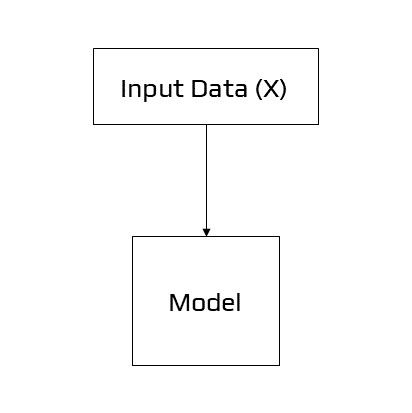
Another learning approach is one in which the model is provided with only the input variables (X) and the challenge has no output variables (y). The patterns in the dataset are extracted or summarised to create a model. Because the model isn’t forecasting anything, there isn’t any need for it to be corrected.
Example of Unsupervised Learning
The unsupervised learning technique [7] is the second primary form of machine learning. The aim is to discover “meaningful findings” in the data, and we are only provided inputs. Because we are not informed what sorts of patterns to look for and there is no clear error measure to utilize, this is a far less well-defined problem unlike supervised learning, where we can compare our predicted y for a given x to the observed value, unsupervised learning does not allow us to compare our predictions to the observed value. Unsupervised learning is the term used to describe this lack of correction. Clustering and generative modelling are examples of unsupervised learning problems, whereas K-means and Generative Adversarial Networks are examples of unsupervised learning algorithms.
Discriminative and Generative Modelling
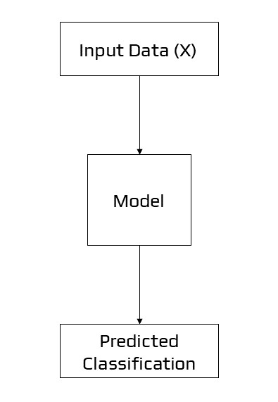
We could be interested in creating a model that predicts a class label given a sample of input variables in supervised learning. This process of predictive modelling is known as classification.
Example of Discriminative Modelling
Discriminative modelling and classification are two terms that have been used interchangeably in the past. We combine the inference and evaluation stages into a single learning problem by using the training data to develop a discriminant function f(x) that maps each x directly onto a class label. This is because a model must distinguish between instances of input variables belonging to different classes; it must pick or decide which class a given example belongs to. A discriminative model overlooks the question of whether or not a particular event is likely, instead of focusing on the likelihood of a label being applied to it.
Example of Generative Modelling
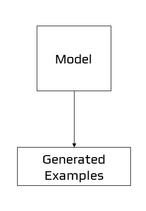
Unsupervised models that summarise the distribution of input variables, on the other hand, could be able to produce or generate new examples in the distribution. As a result, generative models are used to describe various sorts of models. A single variable, for example, could have a well-known data distribution, such as a Gaussian distribution or a bell curve. A generative model may be able to adequately describe this data distribution and then be used to create new variables that fit within the input variable’s distribution.
Generative models are approaches that explicitly or implicitly describe the distribution of inputs and outputs, allowing synthetic data points to be generated in the input space by sampling from them. A competent generative model may be able to produce new instances that are not just reasonable, but also indistinguishable from real-world examples.
A generative model takes into account the data’s distribution and informs how likely a specific occurrence is. Because they can assign a probability to a succession of words, models that predict the next word in a sequence are often generative.
Generative models Examples
Naive Bayes [8] is a generative model that is frequently used as a discriminative model. Naive Bayes sums together the probability distributions of each input variable and the output class. When making a prediction, the chance of each potential outcome for each variable is computed, the independent probabilities are added, and the most likely outcome is predicted. Using the probability distributions for each variable in reverse, new reasonable (independent) feature values may be generated. Latent Dirichlet Allocation [9] (LDA) and the Gaussian Mixture Model [10] (GMM) are two more examples of generative models.
As generative models, deep learning approaches can be employed. The Restricted Boltzmann Machine [11] (RBM) and the Deep Belief Network [12] (DBN) are two prominent examples. The Variational Autoencoder [13] (VAE) and the Generative Adversarial Network (GAN) are two examples of deep learning generative modelling techniques that are currently in use.
Overview of GAN Structure
There are two elements to a generative adversarial network (GAN):
- The generator improves its ability to create credible data over time. The discriminator uses the produced instances as negative training examples.
- The discriminator learns to tell the difference between false and real data generated by the generator. The generator is penalised by the discriminator if it produces improbable results.
When training begins, the generator generates false data, which the discriminator soon recognises:
The generator comes closer to creating output that can deceive the discriminator as training progresses:
Finally, assuming generator training goes well, the discriminator becomes less capable of distinguishing between genuine and fake objects. It begins to mistakenly identify false data as real, and its accuracy suffers as a result.
The following is a diagram of the entire system:
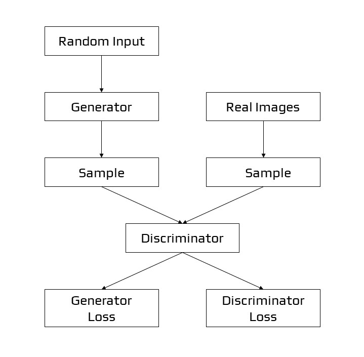
Structure of GANs
The Generator
By integrating input from the discriminator, the generator portion of a GAN learns to produce false data. It learns how to convince the discriminator that its output is real.
Generator training necessitates a greater degree of integration between the generator and the discriminator than discriminator training. The component of the GAN that trains the generator consists of the following:
- random input
- The random input is transformed into a data instance via the generator network.
- The produced data is classified using a discriminator network.
- discriminator output
- Generator loss is a penalty imposed on the generator when it fails to mislead the discriminator.
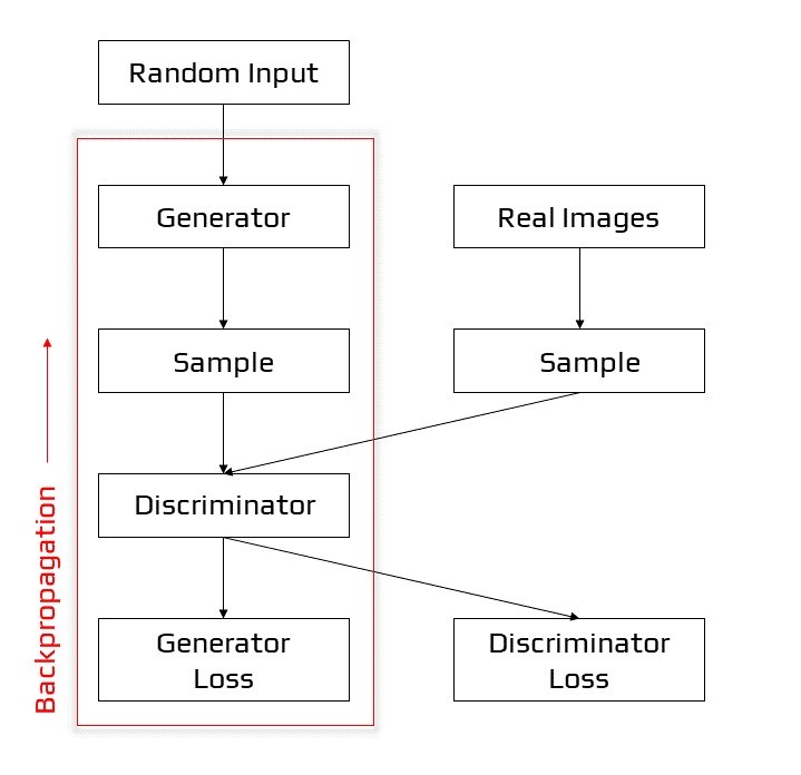
Backpropagation in generator training
Random Input
In order to function, neural networks require some type of input. We usually enter data that we wish to do something with, such as a case that we want to categorise or forecast. What, on the other hand, do we feed into a network that generates whole new data instances?
A GAN uses random noise as its input in its most basic form. The generator then converts the noise into something useful. We can get the GAN to create a broad range of data by adding noise and sampling from different points in the target distribution.
Experiments show that the noise distribution is unimportant, therefore we may select a distribution that is simple to sample from, such as a uniform distribution. The space from which the noise is sampled is generally less in size than the dimensionality of the output space for practical reasons.
Training the Generator with the Discriminator
We change the weights of a neural net to decrease the inaccuracy or loss of its output when training it. The generator in our GAN, on the other hand, is not directly related to the loss we are attempting to reduce. The generator feeds into the discriminator net, which generates the output we are seeking to influence. The generator is penalised by the generator loss if the discriminator network classifies a sample as fraudulent.
Backpropagation [14] must incorporate this additional network segment. Backpropagation corrects each weight by estimating the weight’s influence on the output, or how the output would change if the weight were altered. The impact of a generator weight, on the other hand, is determined by the impact of the discriminator weights into which it feeds. As a result, backpropagation begins at the output and flows back into the generator through the discriminator.
During generator training, however, we do not want the discriminator to alter. Attempting to strike a moving target would make an already difficult task considerably more difficult for the generator.
As a result, we use the technique below to train the generator:
- Sample random noise.
- Using sampled random noise, generate generator output.
- For generator output, use the discriminator to classify it as “Real” or “Fake”.
- Calculate the loss incurred as a result of discriminator classification.
- Gradients may be obtained by backpropagation through the discriminator and generator.
- To just modify the generator weights, use gradients.
This is one iteration of generator training.
The Discriminator
In a GAN, the discriminator is essentially a classifier. It tries to tell the difference between actual data and data generated by the generator. Any network architecture suited to the sort of data it’s categorising might be used.
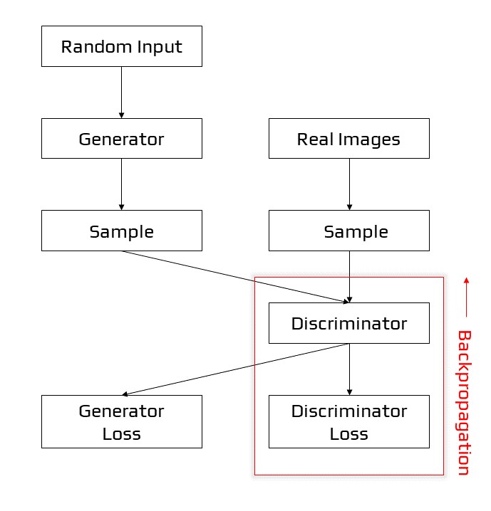
Backpropagation in discriminator training
Discriminator Training Data
The training data for the discriminator originates from two places:
- Real-world data examples, such as real-world portraits of people. During training, the discriminator utilises these examples as positive examples.
- The generator generates fake data objects. During training, the discriminator utilises these events as negative examples.
The generator does not train during discriminator training. It keeps its weights constant while creating samples for the discriminator to learn from.
Training the Discriminator
Two loss functions are connected to the discriminator. The discriminator ignores the generator loss and only utilises the discriminator loss during training. During generator training, we utilise the generator loss.
During discriminator training, the discriminator sorts the generator’s actual and false data. The discriminator suffers a loss if it incorrectly classifies a genuine instance as fake or a fake instance as real. Backpropagation from the discriminator loss across the discriminator network updates the weights of the discriminator.
Training of GAN
The GAN training technique comprises concurrent training of both the discriminator and generator models. The algorithm is summarised in the image below, which is borrowed from Ian Goodfellow and his colleagues 2014 publication titled “Generative Adversarial Networks.”
A summary of the Generative Adversarial Network Training Algorithm.
Algorithm: Minibatch Stochastic Gradient Descent Training of Generative Adversarial Nets
The number of steps to apply to the discriminator, k, is a hyperparameter. We used k = 1, the least expensive option, in our experiments.
for number of training iterations do
for k steps do
Sample minibatch of m noise samples {z(1), ..., z(m)} from noise prior pg(z).
Sample minibatch of m examples {x(1), ..., x(m)} from data generating distribution pdata(x).
Update the discriminator by ascending its stochastic gradient:
end for
Sample minibatch of m noise samples {z(1), ..., z(m)} from noise prior pg(z).
Update the generator by descending its stochastic gradient:
end for
The gradient-based updates can use any standard gradient-based learning rule. We used momentum in our experiments.
The algorithm’s outer loop iterates over steps to train the models in the architecture. One cycle through this loop is not an epoch; rather, it is a single update consisting of particular batch modifications to the discriminator and generator models. An epoch is defined as one cycle through a training dataset in which the samples are utilised to update the model weights in mini-batches. A training dataset of 100 samples used to train a model with a mini-batch size of 10 samples, for example, would result in 10 mini-batch updates for each epoch. The model would be appropriate for a specific number of epochs, such as 500. This is frequently concealed from you by automating model training by calling the fit() method and setting the number of epochs and the size of each mini-batch.
Convergence
Because the discriminator can’t detect the difference between genuine and false, as the generator improves with training, the discriminator’s performance deteriorates. The discriminator has a 50% accuracy if the generator succeeds flawlessly. To make its forecast, the discriminator essentially flips a coin. This development causes difficulty for the GAN’s overall convergence: the discriminator feedback becomes less useful over time. If the GAN continues to train after the discriminator has given totally random feedback, the generator will begin to train on garbage feedback, and its own quality will deteriorate. Convergence is generally a transitory rather than a permanent condition for a GAN.
GAN Loss Functions
The discriminator has been trained to distinguish between authentic and false pictures. This is accomplished by averaging over each mini-batch of samples the log of the anticipated probability of actual pictures and the log of the inverted probability of false images. Remember that adding log probabilities is the same as multiplying probabilities, but without the possibility of disappearing into small values. As a result, we may interpret this loss function as seeking probability near 1.0 for actual pictures and probabilities near 0.0 for false images, inverted to produce bigger numbers. The combination of these numbers indicates that lower average values of this loss function result in higher discriminator performance.
The loss of the generator model is defined by the GAN method as reducing the log of the inverted probability of the discriminator’s prediction of false pictures over a mini-batch. This is simple, but the authors claim that it is ineffective in practice when the generator is weak and the discriminator is skilled at rejecting false pictures with high confidence. The loss function saturates rather than providing appropriate gradient information for the generator to change weights.
Instead, the authors suggest increasing the log of the discriminator’s anticipated likelihood of detecting false pictures. The transformation is slight. In the first example, the generator is taught to reduce the likelihood that the discriminator would be right. With this modification to the loss function, the generator is trained to maximise the likelihood that the discriminator will be wrong. This loss function’s sign may then be reversed to provide a familiar minimising loss function for training the generator. As a result, this is also known as the -log D technique for training GANs.
Loss Functions
GANs are algorithms that attempt to duplicate a probability distribution. As a result, they should utilise loss functions that represent the distance between the GAN-generated data distribution and the distribution of the real data.
In GAN loss functions, how can you represent the difference between two distributions? This is a hotly debated topic, and a variety of techniques have been offered. Here, we’ll look at two typical GAN loss functions that are both implemented in TF-GAN:
- The loss function employed in the study that first described GANs was called minimax loss.
- The default loss function for TF-GAN Estimators is the Wasserstein loss. A 2017 publication was the first to describe it.
TF-GAN also provides a variety of additional loss functions.
Minimax Loss
The generator seeks to reduce the following function, whereas the discriminator strives to maximise it, according to the study that first proposed GANs:
In this function:
- D(x) is the discriminator’s assessment of the likelihood of whether a genuine data instance x exists.
- Ex is the average of all real-world data occurrences.
- G(z) is the outcome of the generator for input noise z.
- D(G(z)) is the discriminator’s estimation of the likelihood that a false example is genuine.
- Ez is the estimated value across all provided by particular inputs (the expected value across all produced false instances G(z)).
- The calculation is based on the difference in entropy between both the real and produced distribution.
- The generator has no significant influence on the log(D(x)) term.
GANs and Convolution Neural Networks
Convolutional Neural Networks [15], or CNNs, are used as the generator and discriminator models in GANs, which generally deal with picture data. This could be due to the fact that the technique was first described in the field of computer vision and used CNNs and image data, as well as the remarkable progress made in recent years using CNNs more broadly to achieve state-of-the-art results on a variety of computer vision tasks like object detection and face recognition. When the latent space, the generator’s input, is used to model picture data, it offers a compressed representation of the collection of images or photographs used to train the model. It also implies that the generator creates fresh pictures or photographs, resulting in an output that developers or users of the model can readily examine and evaluate. It’s possible that this characteristic, above all others, the capacity to visually judge the quality of the produced output, has both led to the emphasis of computer vision applications with CNNs and to the huge jumps in capabilities of GANs when compared to other generative models, deep learning-based or not.
Variations of GANs
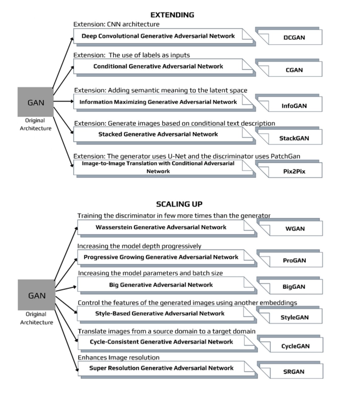
Types of GAN Model architectures and extensions
Deep Convolutional GAN
DCGAN [16] is an expansion of the GAN system that uses deep convolutional neural networks for both the generator and discriminator models, as well as model and training settings that result in robust training of a generator model. DCGANs employ stride and fractionally stride convolutions which are basic blocks of convolution that are used in CNN. This enables the model to learn about the operators used in up sampling and down sampling networks all through the training. Up sampling is expanding the conceptual images representations through multiple techniques to keep the spatial dimensions comparable to the input data. Down sampling is the loss of spatial resolution yet maintaining the same two-dimensional image representation.
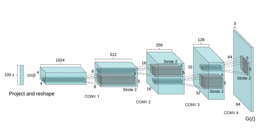
The DCGAN generator was used to simulate the LSUN scenario. A 100-dimensional uniform distribution Z is projected to a limited spatial extent convolutional representation with numerous feature maps. This high-level representation is then converted into a 64 × 64-pixel picture via a sequence of four fractionally-strided convolutions (in some recent studies, they are incorrectly called deconvolutions). It is worth noting that no completely linked or pooling layers are employed.
Conditional GAN
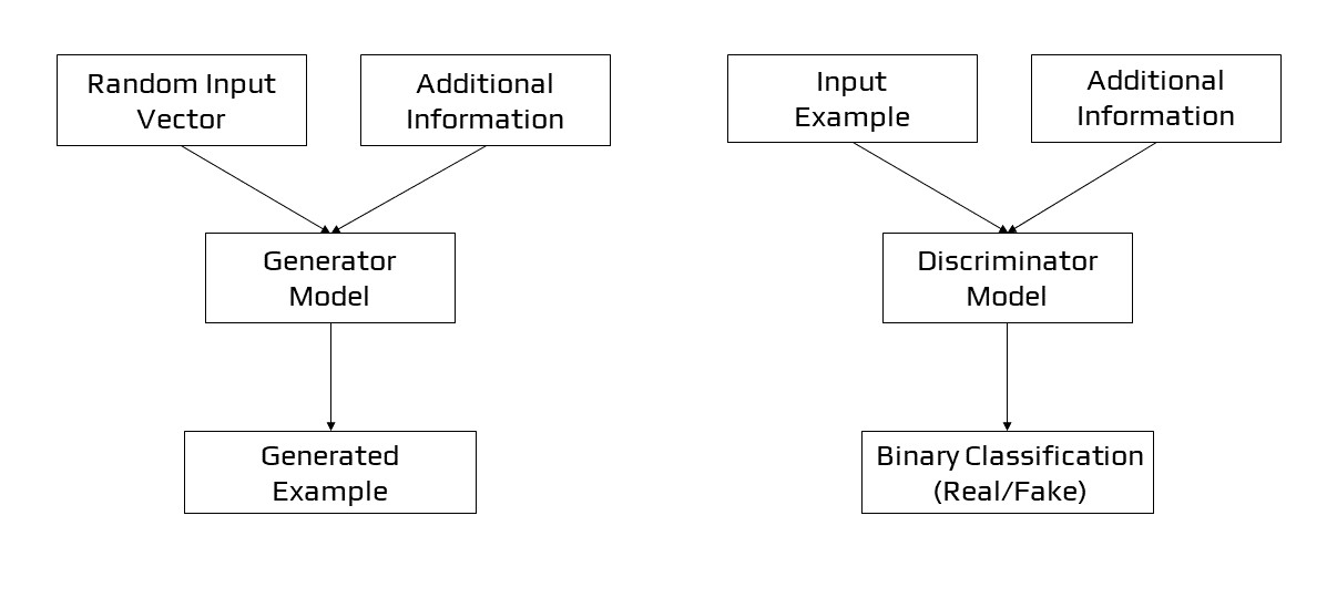
Conditional GANs [17] (cGANs) are a type of network where both the generator and discriminator are conditioned by extra information during training. cGANs modify the network by introducing the label y as an extra argument to the generator so that the generator can produce matching pictures. Labels are also fed to the discriminator to improve the discrimination between real and fake samples. Conditional GANs use a labelled data set to train and allow to choose the label for each produced instance. An unconditional MNIST GAN, for example, will create random digits, but a conditional MNIST GAN will allow us to select which digit the GAN should generate. Conditional GANs represent the conditional probability P(X | Y) instead of the joint probability P(X, Y).
The use of the GAN for conditionally producing an output is a significant extension. The generative model may be trained to create new instances from the input domain, where the input, a random vector from the latent space, is supplemented (conditioned by) some extra information. In the case of producing photos of handwritten numbers, the extra input may be a class value, such as male or female in the case of generating photographs of humans, or even a figure in the event of photographing handwritten characters. If both the generator and the discriminator are conditioned on some additional information y, such as class labels or input from other modalities, generative adversarial networks can be expanded to a conditional model. We may do the conditioning by adding y as an additional input layer to both the discriminator and the generator.
The discriminator is additionally conditioned, which means it is given both a genuine and a false input picture as well as the additional input. The discriminator would therefore anticipate the input to be of that class in the case of a classification label type conditional input, training the generator to create instances of that class in order to mislead the discriminator. A conditional GAN may be used in this way to produce examples from a domain of a specific type.
GAN models can be conditioned on a domain exemplar, such as a picture, if taken a step further. This enables GANs to be used in applications such as text-to-image or image-to-image translation. This enables GANs to do some of their most spectacular tasks, such as style transfer, photo colourization, and photo transformations from summer to winter or day to night, among others.
When using conditional GANs for image-to-image translation, such as converting day to night, the discriminator is fed samples of actual and produced night-time pictures, as well as (conditioned on) real daytime photos. A random vector from the latent space, as well as (conditioned on) real daytime photographs, are fed into the generator.
Conditional GAN Model Architecture
Information Maximizing GAN
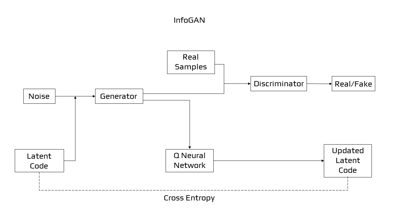
Information Maximizing GAN [18] is a GAN derivative. It’s an algorithm for learning unsupervised representations. This network magnifies the mutual information between the input noise vector and the latent code, which are basically variables that aren’t observed during the training phase and the test phases. InfoGan solves the problem of entangled representations and gives a disentangled one. It separates the Generator input noise vector in two: the conventional noise vector and a new ’latent code’ vector. Later, by maximising the mutual information between the code and the generator output, the latent code is made significant and are used to condition or control specific semantic properties in the generated image. The addition of the component which maximises the mutual information among the generative model’s latent code input and its output, leads to the disentanglement of the significant features and assigns them to the enforced latent code space.
InfoGAN
Stacked GAN
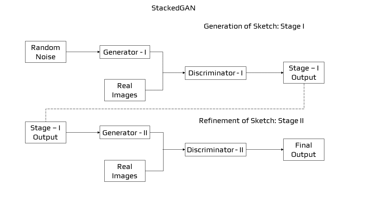
The stacked generative adversarial network, or StackGAN [19][20], is a GAN modification that uses a hierarchical stack of conditional GAN networks to create pictures from words. The structure is made up of conditional GAN models. There are two generators, the first one is text conditioned and produces a poor resolution image. The second one is regulated on the text and the output of the first generator; it produces a high-resolution picture. Our SGAN breaks down variations into several layers and gradually eliminates uncertainties in the top-down generating process, unlike the original GAN, which utilises a single noise vector to represent all variations.
StackGAN
Pix2Pix
The Pix2Pix [21] GAN is a method for teaching convolutional neural networks to do an image-to-image conversion. When compared to previous GAN models (e.g., 256×256 pixels), the precise setup of architecture as a sort of image-conditional GAN provides for both the creation of big pictures and the capacity to perform well on a range of image-to-image machine translation. Pix2Pix is a form of conditional GAN, or cGAN, in which the output picture creation is dependent on input, in this instance a source image. An original picture and a target image are supplied to the discriminator, who must decide if the target is a reasonable translation of the input images.
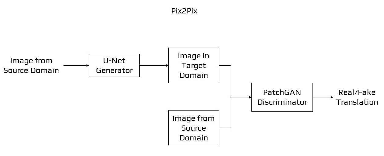
Pix2Pix
Wasserstein GAN
Wasserstein GAN [22] or WGAN is a GAN extension that looks for a different approach to train the generator model so that it can better mimic the distribution of data seen in a particular training dataset. For each iteration, it modifies the training method to update the discriminator model, several times more than the generating model. The discriminator is revised to produce a real-value (linear activation) rather than binary forecasting with a sigmoid function. Both the generator and the discriminator are trained with “Wasserstein loss”. It is the average of the product of real and estimated values from the discriminator to give linear gradients useful for updating the model.
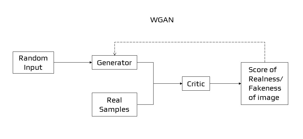
Wasserstein GAN
Progressive Growing GAN
Progressive Growing GAN [23] is a GAN training method enhancement that enables for the steady training of generator networks capable of producing huge, high-quality pictures. The process consists of increasing the size of the model gradually for a very small picture. This will result in a rise in the output size of the generator and the input size of the discriminator. It will continue till the required picture size is obtained. The earliest layers of a progressive GAN create relatively low-quality pictures, but later layers add details. This method allows the GAN to train faster than non-progressive GANs while also producing higher-resolution pictures.
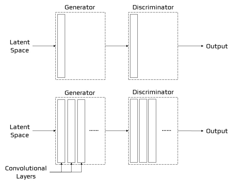
ProGAN
BigGAN
Big Generative Adversarial Networks [24] is a method for demonstrating how existing class conditional models may be scaled up to produce high-quality output pictures. BigGAN is a GAN extension; the idea is to increase the size of the batches while also increasing the amount of parameters. As a result, high-quality, high-resolution images are generated. Modifying the architecture and training procedures, for example, will allow GANs to be scaled up.
StyleGAN
The StyleGAN [25][26], or style-based generative adversarial network, is a generator modification that enables the latent code to be utilised as input at various stages during the model to influence aspects of the produced picture. Rather than using the latent space point as input, the point is passed via a deep embedding system before it can be used as input at numerous places in the generator model. Along with the embedding network’s output, noise is also included.
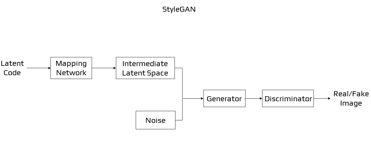
StyleGAN
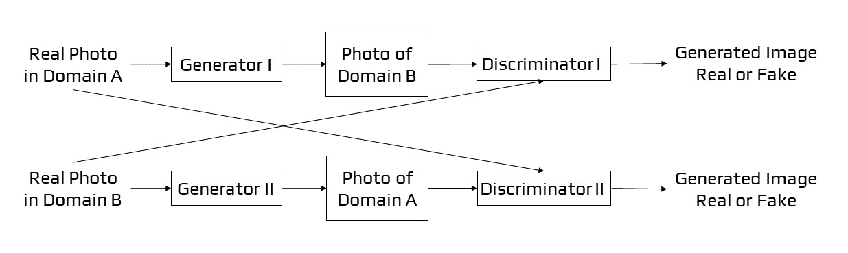
CycleGAN
CycleGANs [27] are generative adversarial networks with two generators and two discriminators. Every generator has its discriminator that aims to differentiate its generated pictures from genuine ones.
CycleGAN
CycleGANs learn to convert pictures from one set into images that may be from a different collection. When given the left-hand picture as input, a CycleGAN created the right-hand image below. It took a horse image and transformed it into a zebra image. The CycleGAN’s training data consists of just two picture sets (in this case, a set of horse images and a set of zebra images). No labels or pairwise picture correspondences are required by the system.
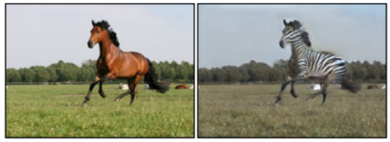
(A) Input Image (B) Output Image
Super-Resolution GAN
Super-Resolution GAN [28], like other GAN designs, is separated into two sections: the generator and the discriminator. The generator generates data based on a probability distribution, and the discriminator attempts to predict if the data came from the input samples or generated samples.
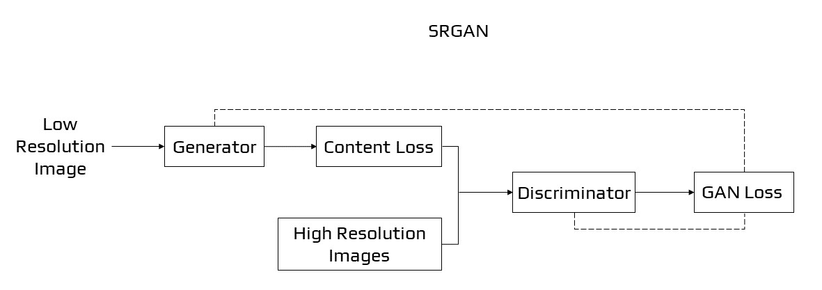
SRGAN
To generate better quality pictures, SRGAN employs a network model in association with an adversarial network. GANs with super-resolution boost picture resolution by adding detail where it’s needed to fill up hazy regions. The fuzzy middle picture on the right, for example, is a down-sampled reproduction of the original image on the left. A GAN created the clearer picture on the right from the fuzzy image:
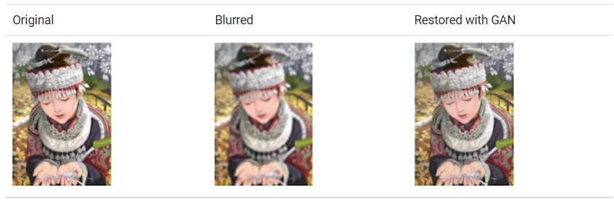
(A) Input Image (B) Blurred (C) Restored with GAN
Although the GAN-generated picture appears to be extremely similar to the original, a careful examination of the headband reveals that the GAN did not replicate the original’s starburst pattern. Instead, it created its own convincing pattern to replace the down-sampled pattern.
Applications of GANs
Exploring recent advances for adversarial deep network training is an ongoing focus of study. Some examples of applications were selected to demonstrate some diverse methods to employ GAN-based representations for picture modification, analysis, or characterisation, and thus do not completely represent the possible range of use of GANs.
Image synthesis [29] is one of the core application GAN functions and it is used when there are some existing conditions for the produced images. Image to Image translation [30] shows the potential of GANs by translating input data into an output image. Super-resolution using GAN demonstrates the use of an existing technique that can be enhanced with supplement loss functions to generate high-quality outcomes.
Image Synthesis
Recently, the research regarding image synthesis with GAN [31] mostly focuses on the quality of the generated images. We can distinguish three approaches for image synthesis: direct, hierarchical, and iterative.
Direct methods are methods in which the models contain a generator G and discriminator D and have a simple architecture with fewer connections. Of these, DCGAN is one of the most traditional, with a framework that is adopted by several subsequent models. In DCGAN, G adopts transposed convolution, batch-normalization and ReLU activation whereas D employs convolution, batch-normalization and Leaky ReLU activation. As its name indicates, this method is very direct for designing and implementing. DCGAN was implemented for the generation of apparel pictures for inclusion in the Fashion MNIST dataset. In this case, the noise was given as input to the generator, then moulded to produce a low image resolution. To obtain the final picture, this was up-sampled using Conv2DTranspose. The discriminator had an architecture based on CNN supervised learning for classifying the generated image.
Compared to the direct method, the hierarchical approach uses two pairs of generators and discriminators. Both the generators and discriminators have different purposes. The two generators’ relationship might be either parallel or sequential. In the case of Structure-Style GAN, it contains two GANs, one GAN to create a surface map from latent space and the other one to take both the created surface normal map and a noise vector as input and produce an image.
The Iterative method is different from the Hierarchical method. This method uses several generators with similar structures and the generators produce images from rough to detailed, with the generators improving the previous output each and every time. Furthermore, for the architecture of the generators, shared weights can be employed between the generators. This however is not possible in the case of hierarchical models. For example, Text-to-Image synthesis, the text is used as input and the model generates pictures that are believable and accurately represented by the text. For text-to-image synthesis, StackGAN suggests using two distinct generators. The first generator produces low-quality images with rough forms and colors of objects. The second one takes as input the outcome of the previous generator and generates high-quality images. The floral image below, for example, was created by feeding a written description to a GAN.
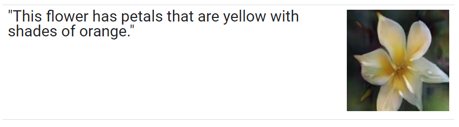
The floral image above was created by feeding a written description to a GAN.
Image-to-Image Translation
The challenge of converting a potential representation of one image into the other, such as transforming black and white pictures into RGB images, or the other way around, is characterised as image-to-image translation. Image-to-image is not limited only to translating the images but also changing and modifying the characteristics of the images. GANs take an input image and map it to a produced output image with various characteristics. Based on the data, we can say that there are two types of translation, supervised and unsupervised.
In Supervised translation, there are paired images in several domains. It means that for each image of the source domain, there exists a corresponding image in the target domain. Pix2Pix merges the loss of a cGAN with the loss of L1 regularization for the generator to fool the discriminator but also produce actual, real images. Though Pix2Pix generates highly amazing synthetic pictures, its main restriction is that it must take coupled photos as supervision, because the data pair (x, y) is taken from the joint distribution p(x, y). Another image-to-image translation case is the White Box Cartoonization using extended GAN framework [32][33]. This network outputs a cartooned image from a given photo. The image is separated in three representations: surface, structure and texture representations. The first one smoothens the surface of the image, the second one segments the image and create a segmentation map. The third one focuses on the colors and the texture as it name indicates. The output is a high resolution and high-quality cartooned image which is very similar to the original photo, yet holds the characteristics of a cartooned picture.
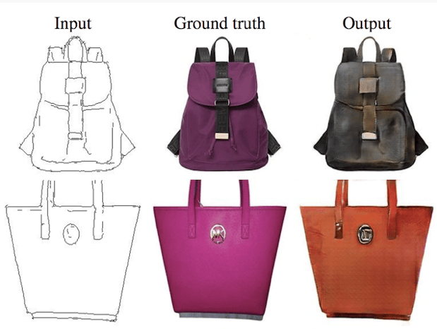
(A) Input Images (B) Real Images (C) Output Images
In an Unsupervised setup [34][35], there are two independent datasets: one has images from one domain while the other has images from another. Consequently, there is no paired data. This poses a challenge as there is no way of showing how the image could be translated into its respective image of another domain. The goal of unsupervised image-to-image translation is to learn a joint distribution of pictures in distinct domains by taking pictures from the probability distribution in each domain. Adversarial Open Domain Adaptation for sketch-to-photo synthesis [36] is a framework that has dealt with unsupervised translation. It uses two generators, G1 translates photo to sketch and G2 translates sketch to photo depending on the input tag, and two discriminators D1 and D2 for drawing and photo domains.
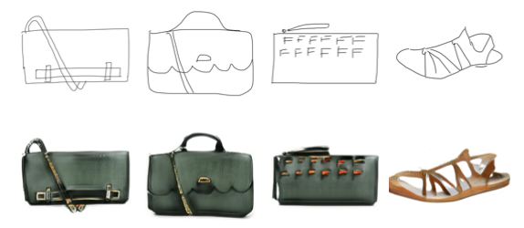
Sketch-to-Photo Synthesis
Conclusions
GANs are a type of game-theoretic generative model. They’ve had a lot of success in the field of creating realistic data, particularly pictures. Training them is still a challenge. It will be required to create models, prices, or training algorithms that can consistently and rapidly identify appropriate Nash equilibria for GANs in order for them to become a more dependable technology. GANs have inspired a surge of interest due to their capacity to learn deep, highly non-linear mappings from a latent space to data space and back, as well as their ability to handle huge amounts of unlabelled picture data that are inaccessible to deep representation learning. There are several chances for theoretical and algorithmic advancements within the intricacies of GAN training, and with the strength of deep networks, there are numerous opportunities for new applications. By creating their own representations of the data they are trained on, GANs produce organised geometric vector spaces for a variety of domains. GANs may train representations that can be used for a variety of tasks, including image synthesis, semantic image editing, style transfer, image super-resolution, and classification, to name a few applications.
Additional Resources
Research Paper
Explore the published research paper and preprint:
Citation
Please cite this work as:
Thakur, Amey. "Generative Adversarial Networks". AmeyArc (Aug 2021). https://amey-thakur.github.io/posts/2021-08-27-generative-adversarial-networks/.Or use the BibTex citation:
@article{thakur2021gan,
  title   = "Generative Adversarial Networks",
  author  = "Thakur, Amey",
  journal = "amey-thakur.github.io",
  year    = "2021",
  month   = "Aug",
  url     = "https://amey-thakur.github.io/posts/2021-08-27-generative-adversarial-networks/"
}